
Archive for the ‘general math’ Category
While I was away the 32nd carnival of Mathematics was posted over at TCMTB. This edition might be small but it is perfectly formed with articles on topics such as the combinatorics of words and a nice variation on Tic Tac Toe.
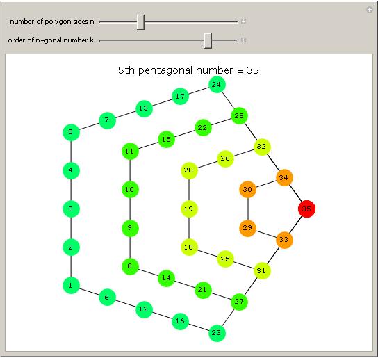
The 31st edition of the Carnival of Mathematics is up over at Recursivity. As always, there is a wide variety of material of offer with everything from recreational mathematics through to graduate level stuff. I liked the post on figurative numbers by Denise over at Let’s play math because I recently read about them in the book Recreations in the Theory of Numbers by Arthur Beiler. For a moment I thought it would be fun to write a Wolfram Demonstration about figurative numbers but it’s already been done – oh well, never mind. Enjoy the carnival.
In the recent 30th edition of the Carnival of Mathematics, the author mentioned that 30 is the first Sphenic number. I had never heard the term before so I thought I would investigate them a bit – nothing serious, just a bit of googling. The Wikipedia page was the first hit and this told me that Sphenic Numbers are positive integers that are the product of three distinct primes.
The article also demonstrated that Sphenic Numbers have exactly 8 divisors and gave some other bits of trivia such as the largest known example of a Sphenic Number (the product of the 3 largest known primes). There was also a link to the sequence of sphenic numbers on The On-Line Encyclopedia of Integer Sequences and that was about it. Oddly for something so elementary – there was nothing about Sphenic Numbers on Mathworld although this may change now that my Wolfram Demonstration on Sphenic Numbers has been published.
I was curious about what had written about Sphenic numbers in the literature so I googled the term on Google Scholar – amazingly there was not a single hit. So it seems that these numbers were considered important enough by someone to give them their own name but no one has then used that name in the literature….EVER!
How about books? Searching for “Sphenic Numbers” in Google Books also results in no hits. “Sphenic Number” results in one hit for a book called “Worlds of If” – No preview is available and the only quote you can get is “A sphenic number is one with unequal factors”
So – Where on earth did the name come from? Wikipedia says that its from the old greek word ‘sphen’ which means wedge but what I really want to know is who first gave these numbers this name? Why are there no references to the name in the literature? Does anyone know any interesting theorems concerning Sphenic Numbers?
Finally, is there a name for numbers that are the product of 4 distinct primes, or 5, or 6?
I am just about to go into hospital to have my wisdom teeth removed under general anesthetic, but before I go I thought I would mention that I have discovered an elementary proof of the Riemann Hypothesis and will share it with you all as soon as I get back.
Update – 11th April 2008
Of course I have not proved the Riemann Hypothesis at all but I was a bit worried about having that general anesthetic and so, following the example of Godfrey Harvey, I thought I would take out a little health insurance ;)
The minimization of the Rosenbrock function is a classic test problem that is extensively used to test the performance of different numerical optimization algorithms. It was first introduced in 1960 by H.H Rosenbrock in his paper, “An Automatic Method for Finding the Greatest or Least Value of a Function, Computer J. 3, 175-184, 1960 (See here for Rosenbrock’s account of how he came to write that paper.)
The function definition is given below and, although it looks harmless enough, it turns out to be quite challenging to find it’s minimum point by numerical methods.

Acording to Google Scholar, Rosenbrock’s paper has been cited no less than 596 times (as of April 9th 2008) and the function he introduced has been used as a test problem for many different numerical solvers including those in the Matlab Optimization toolbox, The NAG libraries, COMSOL and SciPy (A python module).
So why is this innocuous looking function so difficult to minimise? To answer that let’s first take a look at its contour plot using Mathematica.
ContourPlot[(1 – x)^2 + 100 (y – x^2)^2, {x, -2, 2}, {y, -2, 2},
ContourShading -> False, Contours -> Table[10^-i, {i, -2, 10, 0.5}]
, Epilog -> {Black, PointSize[Large], Point[{1, 1}]}]
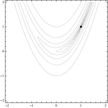
The global minimum of the Rosenbrock function lies at the point x=1, y=1 and is shown in the above diagram by a black spot. Note that the contours are not evenly spaced in this diagram – they are logarithmically spaced instead so the solution lies inside a very deep, narrow, banana shaped valley. The distinctive shape of this function’s contour lines is the reason for its alternative name – “Rosenbrock’s banana function”.
The valley causes a lot of problems for search algorithms such as the method of steepest descents which will quickly find the ‘entrance’ to the valley and then spend hundreds of iterations zigzagging from one side of it to the other – making very slow progress towards the minimum itself.
There is a Mathematica function called FindMinimum that can handle this kind of optimization problem and I wondered how its methods would handle the Rosenbrock function. In the back of my mind I thought that I might also be able to make a nice Wolfram Demonstration from the investigation. While looking at the documentation for FindMinimum I found an example that pretty much solved the problem for me.
pts = Reap[FindMinimum[(1 – x)^2 + 100 (-x^2 – y)^2, {{x, -1.2}, {y, 1}}, StepMonitor :> Sow[{x, y}]]][[2, 1]];
pts = Join[{{-1.2, 1}}, pts];
This finds the minimum point from a starting point of x=-1.2, y=1 and also stores all of the intermediate steps so you can see the path that Mathematica takes in looking for the solution. The only other piece of information needed was to find out how to specify the solution method. It turns out that this is obvious – just use the option
Method->”MethodNameHere”
replacing MethodNameHere with whatever method you want Mathematica to use. You can choose from ConjugateGradient, LevenbergMarquardt, Newton, QuasiNewton, PrincipalAxis and InteriorPoint.
All that remained was to wrap this up in a Manipulate statement, make it look pretty, add some controls and submit it to the demonstrations project. The result can be found here.
One of the things I like about the process of submitting demonstrations to the project is that they are refereed. Someone will take the time to look at your code and make suggestions and small modifications before it gets published. This reduces the possibility of mistakes being made in the final version and really helps with the learning process. Almost every time I have submitted something, I have learned a little more about Mathematica – and that’s really the main reason for me doing it (well its also fun to have your name “up in lights” if I am being honest).
At this point I would like to thank the members of the Wolfram Demonstrations team who have dealt with my submissions so far – not only have they been a pleasure to work with and extremely patient but they have also spared my blushes by pointing out some very stupid mistakes in my code. Of course any that remain are my fault and not theirs.
The 29th edition of the Carnival of Mathematics has been posted over at quomodocumque. Topics include group theory, game theory, the Collatz conjecture and much more.
In a recent post I asked if anyone had any requests for any Wolfram Demonstrations that they would like to see made. Maria Andersen of the Teaching College Math Technology Blog requested a demonstration that would produce music from the decimal expansion of rational numbers in the same way that this one does for irrational numbers. Well, I always aim to please so here it is:
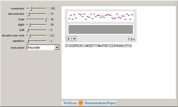
Just set the numerator and denominator with the sliders, choose the base of the result, the number of digits etc, along with what instrument you want and then click play. Remember, if you don’t have Mathematica then you can always use their free MathPlayer to run this demonstration. I hope this is what you were looking for Maria but if it isn’t then let me know what you would like changed and I will see what I can do.
If anyone else has any Wolfram Demonstration requests then leave a comment and I might just code it up for you (unless someone beats me to it of course).
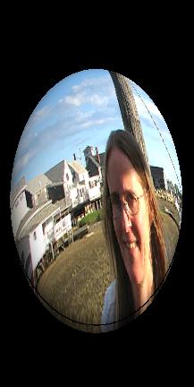
1.Take one dare from Kathryn Cramer and obtain a picture from her website.
2. Steal ideas from this demonstration by Jeff Bryant.
3. Type the following incantations into Mathematica
SetDirectory[“/home/mike/Desktop/random”];
image = Import[“kramer.jpg”];
xpos[x_] := Floor[x/N[2/374.] + 377/2.]
ypos[x_] := Floor[x/N[2/499.] + 502/2.]
imcol[x_, y_] := image[[1]][[1]][[xpos[x]]][[ypos[y]]]/256.;
a = 1; b = 0.9; c = 1;
Plot3D[{Sqrt[ c^2*(1 – (x^2/a^2 + y^2/b^2))], -Sqrt[c^2*(1 – (x^2/a^2 + y^2/b^2))]}, {x, -1, 1}, {y, -1, 1}, ColorFunction -> (RGBColor[imcol[#1, #2]] &), Boxed -> False, Axes -> False, AspectRatio -> 2, ViewAngle -> Pi/13, ViewPoint -> {-3.00336, 0.86708, 3.14159}, PlotRange -> All, Mesh -> False, PlotPoints -> 400]
Enjoy!
Next Friday will be March 14th which is celebrated by some as Pi Day since the date is 3/14 in American date format and the first three digits of Pi are 3.14 (as if I have to tell you!). One or two people have been looking for inspiration as to what to do for Pi Day in schools and I thought that it would be fun to write a Wolfram Demonstration especially for Pi Day, after all, my Valentine’s day demonstrations turned out to be quite popular.
So the question that remained to be answered was “what demonstration should I write?”
I have already written a post about making music out of the digits of Pi and discovered that a great demonstration had been written by Hector Zenil so there was no point in thinking about that.
How about Buffon’s needle? That’s a fun problem that leads to an approximation of Pi. Unfortunately for me – this is a demonstration that has already been written.
Perhaps I could do something that looked at the randomness in the digits of Pi? After all – this blog IS called walking randomly and I haven’t looked at randomness very much yet. Unfortunately I have been beaten to this one too (By Stephen Wolfram himself no less).

My next thought was to consider some series that would sum up to approximations of Pi. Again – it’s been done.

In addition to these three there are many others such as
- Consecutive Digits in the Expansion of Pi
- Pi Digits Bar Chart
- Pi Digits Pie
- Wallis’ Sieve Pi Approximation
- Graphs Of Successive Digits Of Pi, E and Phi
- Wallis Formula
That’s a lot of Pi and I have only just gotten started. All in all I am stumped – I have no idea of a demonstration I might write for Pi Day but if you can think of something then let me know and I will see what I can do :) (Oh and I will make sure that you get credit for your idea when I submit it to the project)
A couple of weeks ago I started thinking about Valentine’s day and, since I like equations that have interesting plots so much, I wondered if I could find one that had a heart-shaped graph. A quick google search came up Wolfram Research’s Heart Surface page.
The main page described a couple of heart shaped algebraic surfaces which looked nice but there were a few more on the Mathematica notebook that the page linked to. This notebook was rather old and included plots from old versions of Mathematica so on the train ride home I wrapped these equations in some Manipulate functions and sent the resulting demo to Wolfram. The result was published today on the Wolfram Demonstrations site.

Essentially all this demo does is use Mathematica’s ContourPlot3D function to plot the curves formed from the following equations and allow you to play with the results a bit.
Nordstrand

Kuska

Taubin

Trott

Each equation is named after the person who first wrote it down (to my knowledge at least). It’s a simple demo but I hope you like it.
Happy Valentine’s day.