
Archive for the ‘just for fun’ Category
Consider this indefinite integral

Feed it to MATLAB’s symbolic toolbox:
int(1/sqrt(x*(2 - x)))

ans =
asin(x - 1)
Feed it to Mathematica 8.0.1:
Integrate[1/Sqrt[x (2 - x)], x] // InputForm

(2*Sqrt[-2 + x]*Sqrt[x]*Log[Sqrt[-2 + x] + Sqrt[x]])/Sqrt[-((-2 + x)*x)]
Let x=1.2 in both results:
MATLAB's answer evaluates to 0.2014
Mathematica's answer evaluates to -1.36944 + 0.693147 I
Discuss!
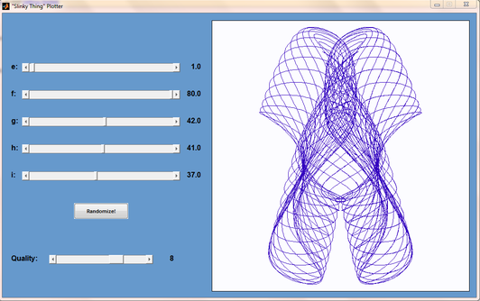
Matt Tearle has produced a MATLAB version of my Interactive Slinky Thing which, in turn, was originally inspired by a post by Sol over at Playing with Mathematica. Matt adatped the code from some earlier work he did and you can click on the image below to get it. Thanks Matt!
This lunchtime I stumbled across the following tweet by GrrlScientist
“mmm, cheese! RT @LookMaNoFans How many Calories would a Moon made of cheese be, you ask? A made-of-manchego Moon = 285 septillion Calories.”
A septillion is 10^24 so that’s a lot of calories! Naturally, I wanted to check the facts so I asked Wolfram Alpha which, sadly, didn’t have the specifics on manchego cheese so I substituted monterey cheese to get a result of 8.5*10^25 calories. This disagrees with the tweet but it’s the figure I’m going to go with for now.
Since I am into running, I wondered how far I’d have to run to burn that many calories. Using Wolfram Alpha’s running calorie calculator I found out that at a pace of 8 minutes per mile I would need to run 0.675 miles to burn 85 calories (assuming average body weight*) so would need to run 6.75*10^24 miles (almost 115 billion light years) to burn off the calories contained in a moon made of monteray cheese. That’s larger than the diameter of the observable universe!
*Obviously, if you ate the moon then you would weigh slightly more than average so this is a gross over-simplification.
Over at Playing with Mathematica, Sol Lederman has been looking at pretty parametric and polar plots. One of them really stood out for me, the one that Sol called ‘Slinky Thing’ which could be generated with the following Mathematica command.
ParametricPlot[{Cos[t] - Cos[80 t] Sin[t], 2 Sin[t] - Sin[80 t]}, {t, 0, 8}]
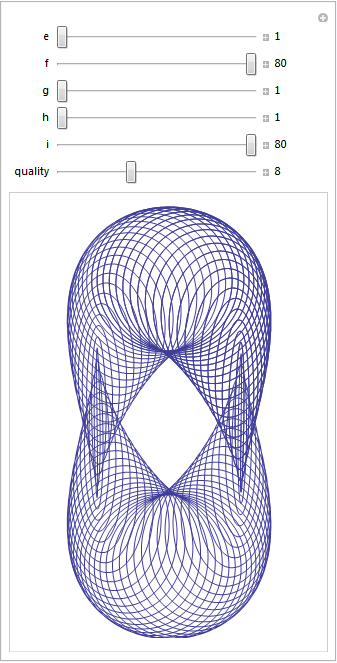
Out of curiosity I parametrised some of the terms and wrapped the whole thing in a Manipulate to see what I could see. I added 5 controllable parameters by turning Sol’s equations into
{Cos[e t] - Cos[f t] Sin[g t], 2 Sin[h t] - Sin[i t]}, {t, 0, 8}
Each parameter has its own slider (below). If you have Mathematica 8, or the free cdf player, installed then the image below will turn into an interactive applet which you can use to explore the parameter space of these equations.
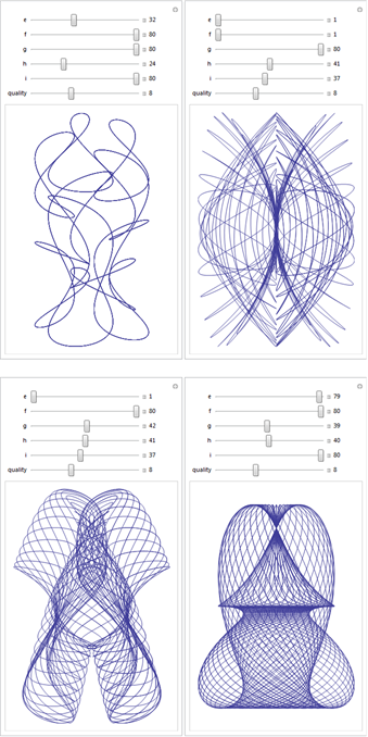
Here are four of my favourites. If you come up with one that you particularly like then feel free to let me know what the parameters are in the comments.
The Pendulum Waves video is awesome and the system has been simulated in Mathematica (twice), Maple and probably every other programming language by now. During a bout of insomnia I used the Mathematica code written by Matt Henderson as inspiration and made a simple MATLAB version. Here’s the video
Here’s the code.
freqs  = 5:15;
num = numel(freqs);
lengths = 1./sqrt(freqs);
piover6 = pi/6;

figure
axis([-0.3 0.3 -0.5 0]);
axis off;
org=zeros(size(freqs));
xpos=zeros(size(freqs));
ypos=zeros(size(freqs));
pendula =  line([org;org],[org;org],'LineWidth',1,'Marker','.','MarkerSize',25 ...
                ,'Color',[0 0 0],'visible','off' );

% Open the avi file
vidObj = VideoWriter('pendula_wave.avi');
open(vidObj);

count =0;
for t=0:0.001:1
    count=count+1;
omegas = 2*pi*freqs*t;
xpos = sin(piover6*cos(omegas)).*lengths;
ypos = -cos(piover6*cos(omegas)).*lengths;

 for i=1:num
 set(pendula(i),'visible','on');
 set(pendula(i),'XData',[0 xpos(i)]);
 set(pendula(i),'YData',[0 ypos(i)]);
 drawnow
 end
 currFrame = getframe;
 writeVideo(vidObj,currFrame)

 F(i) = getframe;
end

% Close the file.
close(vidObj);
I saw a great tweet from Marcus du Sautoy this morning who declared that today, June 28th, is a perfect day because both 6 and 28 are perfect numbers. This, combined with the fact that it is very sunny in Manchester right now put me in a great mood and I gave my colleauges a quick maths lesson to try and explain why I was so happy.
“It’s not a perfect year though is it?” declared one of my colleauges. Some people are never happy and she’s going to have to wait over 6000 years before her definition of a perfect day is fulfilled. The date of this truly perfect day? 28th June 8128.
Update: Someone just emailed me to say that 28th June is Tau Day too!
A while ago I wrote an article on comparing mobile phones with ancient supercomputers and today I learned that Jack Dongarra has run his Linpack benchmark on the iPad 2 and discovered that it has enough processing power to rival the Cray 2; the most powerful supercomputer in the world back in 1985. According to Jack, the iPad 2 is so powerful that it would have stayed in the top 500 list of world’s most powerful super computers until 1994. That’s a lot of power!
Other iPad articles on WalkingRandomly
So here’s a fun (and potentially useful) probability puzzle for you all to ponder. Here in the UK we have an investment option called Premium Bonds. From the premium bonds website:
“Premium Bonds are an investment where, instead of interest payments, investors have the chance to win tax-free prizes. When someone invests in Premium Bonds they are allocated a series of numbers, one for each £1 invested.”
There’s a prize draw every month and a range of prizes from 25 pounds right up to 1 million pounds. You can get your money back at any time with no penalty. So, if you invest 1000 pounds then you get 1000 shots at winning a prize every month for as long as you leave the investment alone. More detailed information such as odds etc is available here.
The way I like to think of premium bonds is that they are a bit like the National Lottery (click here for discussion of odds) except that you get your money back after you’ve played. So I was thinking that, instead of buying premium bonds, an alternative investment strategy would be to put all of your money into a high interest cash account (paying N% per year) and use the resulting interest to buy lottery tickets.
Both strategies offer similar security (you can get your principle investment back at any time) and both of them are a bit of fun since they are based on games of chance. Assuming I am to choose one of these strategies, which one is going to offer me the best rate of return over the long term?
A couple of years ago I wrote an article called Christmas gifts for math geeks and it has proven to be quite popular so I decided to write a follow up. As I started thinking about what I might include, however, I started to realise that I had produced a list for science geeks instead. So, here it is – my recommendations for gifts for the scientist in your life.
Mathematica 8 Home Edition – This is the full version of Mathematica, possibly my favourite piece of mathematical computer software, at the extremely low price of 195 pounds + VAT. I know what you are thinking ‘Over 200 quid is not an extremely low price.’ and I would tend to agree. It is, however, very good value since a commercial license costs several thousand pounds and Mathematica is as good as MATLAB with a whole slew of toolboxes. Mathematica is possibly the most feature complete piece of mathematical software available today and is infinitely better than any dedicated graphical calculator.

Bigtrak – I don’t have a Bigtrak but I used to have one back in the 1980s. Is the science geek in your life into computers and 30-40 years old? If so then there is a distinct possibility that their first foray into the world of computer programming was with a Bigtrak back when they were 8 or so – I mean, this thing can even do loops! This isn’t identical to the original but it is a very close facsimile and would be great for budding computer nerds or their misty eyed old dad.


200-in-1 electronic project lab. Now this one brings back fond memories for me since it was given to me for my 10th birthday and is probably the reason I studied physics at A-Level since A-Level physics included the study of basic electronics. I did well in A-Level physics and enjoyed it so I chose theoretical physics for my degree later moving on to a PhD so you could argue that this piece of kit changed my life!
I was overjoyed when I discovered that it was still being sold and was immensely pleased when I received it as a birthday present once again when I was 28.
The first thing you need to know about this wonderful piece of kit is that it requires no soldering; you wire up all of the components using bendy little springs – nothing could be more simple. There is also no need to be able to read schematic diagrams (although this can be a great way to learn how to) since each spring is numbered so producing your own AM radio transmitter can be as simple as joining spring 1 to spring 10 to spring 53 and so on.
The practical upshot of all of this is that you can approach this thing at a variety of levels. In the first instance you can just have fun building and playing with the various circuits which include things like a crystal set radio, a Morse code transmitter, a light detector, a sound detector and basic electronic games. Once you’ve got that out of your system you can start to learn the basics of electronics if you wish.
I have since discovered 300 in 1


Wonders of the Solar System – I have always loved (although never practised) astronomy and avidly followed the adventures of Voyagers 1 and 2 when I was small. Since then, modern space probes such as Cassini-Huygens, Galileo and Mars Odyssey have added more to our knowledge of our astronomical backyard and we now know a tremendous amount about the solar system. In this series, Brian Cox of the University of Manchester takes us on a grand-tour around the solar system. The imagery is fantastic, Cox’s enthusiasm is infectious and the science is awesome. Yep, I quite like this DVD :)


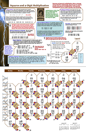
2011 ‘Lightning Calculation’ calendar – Ron Doerfler writes a blog called Dead Reckonings that specialises in the lost arts of the mathematical sciences. Last year he designed a 2010 Graphical Computing calendar and made the designs available for free to allow you to print your own. Centred around ancient computing devices called nomograms, the calendar was beautiful and after Ron very kindly sent me a copy, I encouraged him to make a version that he could sell. Well, I guess he took my advice because Ron is back with a 2011 calendar with the theme of ‘Lightning Calculations’ and this time he is selling it from Lulu.com.
Since Ron is an all round nice guy, he also offers a high resolution pdf of the calendar to allow you to print it off yourself but personally I plan on showing my support by putting an order in with Lulu.com. Nice work Ron!
Some time ago now, Sam Shah of Continuous Everywhere but Differentiable Nowhere fame discussed the standard method of obtaining the square root of the imaginary unit, i, and in the ensuing discussion thread someone asked the question “What is i^i – that is what is i to the power i?”
Sam immediately came back with the answer e^(-pi/2) = 0.207879…. which is one of the answers but as pointed out by one of his readers, Adam Glesser, this is just one of the infinite number of potential answers that all have the form e^{-(2k+1) pi/2} where k is an integer. Sam’s answer is the principle value of i^i (incidentally this is the value returned by google calculator if you google i^i – It is also the value returned by Mathematica and MATLAB). Life gets a lot more complicated when you move to the complex plane but it also gets a lot more interesting too.
While on the train into work one morning I was thinking about Sam’s blog post and wondered what the principal value of i^i^i (i to the power i to the power i) was equal to. Mathematica quickly provided the answer:
N[I^I^I]
0.947159+0.320764 I
So i is imaginary, i^i is real and i^i^i is imaginary again. Would i^i^i^i be real I wondered – would be fun if it was. Let’s see:
N[I^I^I^I]
0.0500922+0.602117 I
gah – a conjecture bites the dust – although if I am being honest it wasn’t a very good one. Still, since I have started making ‘power towers’ I may as well continue and see what I can see. Why am I calling them power towers? Well, the calculation above could be written as follows:

As I add more and more powers, the left hand side of the equation will tower up the page….Power Towers. We now have a sequence of the first four power towers of i:
i = i
i^i = 0.207879
i^i^i = 0.947159 + 0.32076 I
i^i^i^i = 0.0500922+0.602117 I
Sequences of power towers
“Will this sequence converge or diverge?”, I wondered. I wasn’t in the mood to think about a rigorous mathematical proof, I just wanted to play so I turned back to Mathematica. First things first, I needed to come up with a way of making an arbitrarily large power tower without having to do a lot of typing. Mathematica’s Nest function came to the rescue and the following function allows you to create a power tower of any size for any number, not just i.
tower[base_, size_] := Nest[N[(base^#)] &, base, size]
Now I can find the first term of my series by doing
In[1]:= tower[I, 0]

Out[1]= I
Or the 5th term by doing
In[2]:= tower[I, 4]

Out[2]= 0.387166 + 0.0305271 I
To investigate convergence I needed to create a table of these. Maybe the first 100 towers would do:
ColumnForm[
 Table[tower[I, n], {n, 1, 100}]
 ]
The last few values given by the command above are
0.438272+ 0.360595 I
0.438287+ 0.360583 I
0.438287+ 0.3606 I
0.438275+ 0.360591 I
0.438289+ 0.360588 I
Now this is interesting – As I increased the size of the power tower, the result seemed to be converging to around 0.438 + 0.361 i. Further investigation confirms that the sequence of power towers of i converges to 0.438283+ 0.360592 i. If you were to ask me to guess what I thought would happen with large power towers like this then I would expect them to do one of three things – diverge to infinity, stay at 1 forever or quickly converge to 0 so this is unexpected behaviour (unexpected to me at least).
They converge, but how?
My next thought was ‘How does it converge to this value? In other words, ‘What path through the complex plane does this sequence of power towers take?” Time for a graph:
tower[base_, size_] := Nest[N[(base^#)] &, base, size];
complexSplit[x_] := {Re[x], Im[x]};
ListPlot[Map[complexSplit, Table[tower[I, n], {n, 0, 49, 1}]],
 PlotRange -> All]
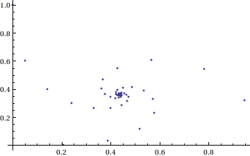
Who would have thought you could get a spiral from power towers? Very nice! So the next question is ‘What would happen if I took a different complex number as my starting point?’ For example – would power towers of (0.5 + i) converge?’
The answer turns out to be yes – power towers of (0.5 + I) converge to 0.541199+ 0.40681 I but the resulting spiral looks rather different from the one above.
tower[base_, size_] := Nest[N[(base^#)] &, base, size];
complexSplit[x_] := {Re[x], Im[x]};
ListPlot[Map[complexSplit, Table[tower[0.5 + I, n], {n, 0, 49, 1}]],
 PlotRange -> All]
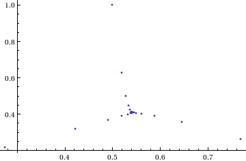 The zoo of power tower spirals
So, taking power towers of two different complex numbers results in two qualitatively different ‘convergence spirals’. I wondered how many different spiral types I might find if I consider the entire complex plane? I already have all of the machinery I need to perform such an investigation but investigation is much more fun if it is interactive. Time for a Manipulate
complexSplit[x_] := {Re[x], Im[x]};

tower[base_, size_] := Nest[N[(base^#)] &, base, size];

generatePowerSpiral[p_, nmax_] :=
  Map[complexSplit, Table[tower[p, n], {n, 0, nmax-1, 1}]];

Manipulate[const = p[[1]] + p[[2]] I;
 ListPlot[generatePowerSpiral[const, n],
 PlotRange -> {{-2, 2}, {-2, 2}}, Axes -> ax,
 Epilog -> Inset[Framed[const], {-1.5, -1.5}]], {{n, 100,
 "Number of terms"}, 1, 200, 1,
 Appearance -> "Labeled"}, {{ax, True, "Show axis"}, {True,
 False}}, {{p, {0, 1.5}}, Locator}]
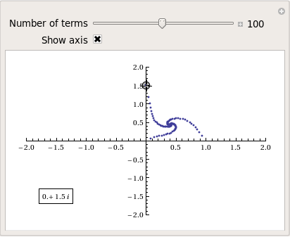
After playing around with this Manipulate for a few seconds it became clear to me that there is quite a rich diversity of these convergence spirals. Here are a couple more
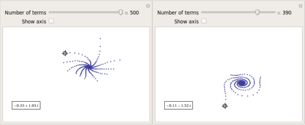
Some of them take a lot longer to converge than others and then there are those that don’t converge at all:
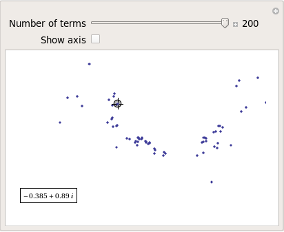
Optimising the code a little
Before I could investigate convergence any further, I had a problem to solve: Sometimes the Manipulate would completely freeze and a message eventually popped up saying “One or more dynamic objects are taking excessively long to finish evaluating……” What was causing this I wondered?
Well, some values give overflow errors:
In[12]:= generatePowerSpiral[-1 + -0.5 I, 200]

General::ovfl: Overflow occurred in computation. >>
General::ovfl: Overflow occurred in computation. >>
General::ovfl: Overflow occurred in computation. >>
General::stop: Further output of General::ovfl will be suppressed during this calculation. >>
Could errors such as this be making my Manipulate unstable? Let’s see how long it takes Mathematica to deal with the example above
AbsoluteTiming[ListPlot[generatePowerSpiral[-1 -0.5 I, 200]]]
On my machine, the above command typically takes around 0.08 seconds to complete compared to 0.04 seconds for a tower that converges nicely; it’s slower but not so slow that it should break Manipulate. Still, let’s fix it anyway.
Look at the sequence of values that make up this problematic power tower
generatePowerSpiral[-0.8 + 0.1 I, 10]

{{-0.8, 0.1}, {-0.668442, -0.570216}, {-2.0495, -6.11826},
{2.47539*10^7,1.59867*10^8}, {2.068155430437682*10^-211800874,
-9.83350984373519*10^-211800875}, {Overflow[], 0}, {Indeterminate,
  Indeterminate}, {Indeterminate, Indeterminate}, {Indeterminate,
  Indeterminate}, {Indeterminate, Indeterminate}}
Everything is just fine until the term {Overflow[],0} is reached; after which we are just wasting time. Recall that the functions I am using to create these sequences are
complexSplit[x_] := {Re[x], Im[x]};
tower[base_, size_] := Nest[N[(base^#)] &, base, size];
generatePowerSpiral[p_, nmax_] :=
  Map[complexSplit, Table[tower[p, n], {n, 0, nmax-1, 1}]];
The first thing I need to do is break out of tower’s Nest function as soon as the result stops being a complex number and the NestWhile function allows me to do this. So, I could redefine the tower function to be
tower[base_, size_] :=
 NestWhile[N[(base^#)] &, base, MatchQ[#, _Complex] &, 1, size]
However, I can do much better than that since my code so far is massively inefficient. Say I already have the first n terms of a tower sequence; to get the (n+1)th term all I need to do is a single power operation but my code is starting from the beginning and doing n power operations instead. So, to get the 5th term, for example, my code does this
I^I^I^I^I
instead of
(4th term)^I
The function I need to turn to is yet another variant of Nest – NestWhileList
fasttowerspiral[base_, size_] :=
 Quiet[Map[complexSplit,
 NestWhileList[N[(base^#)] &, base, MatchQ[#, _Complex] &, 1,
 size, -1]]];
The Quiet function is there to prevent Mathematica from warning me about the Overflow error. I could probably do better than this and catch the Overflow error coming before it happens but since I’m only mucking around, I’ll leave that to an interested reader. For now it’s enough for me to know that the code is much faster than before:
(*Original Function*)
AbsoluteTiming[generatePowerSpiral[I, 200];]

{0.036254, Null}
(*Improved Function*)
AbsoluteTiming[fasttowerspiral[I, 200];]

{0.001740, Null}
A factor of 20 will do nicely!
Making Mathematica faster by making it stupid
I’m still not done though. Even with these optimisations, it can take a massive amount of time to compute some of these power tower spirals. For example
spiral = fasttowerspiral[-0.77 - 0.11 I, 100];
takes 10 seconds on my machine which is thousands of times slower than most towers take to compute. What on earth is going on? Let’s look at the first few numbers to see if we can find any clues
In[34]:= spiral[[1 ;; 10]]

Out[34]= {{-0.77, -0.11}, {-0.605189, 0.62837}, {-0.66393,
  7.63862}, {1.05327*10^10,
  7.62636*10^8}, {1.716487392960862*10^-155829929,
  2.965988537183398*10^-155829929}, {1., \
-5.894184073663391*10^-155829929}, {-0.77, -0.11}, {-0.605189,
  0.62837}, {-0.66393, 7.63862}, {1.05327*10^10, 7.62636*10^8}}
The first pair that jumps out at me is {1.71648739296086210^-155829929, 2.96598853718339810^-155829929} which is so close to {0,0} that it’s not even funny! So close, in fact, that they are not even double precision numbers any more. Mathematica has realised that the calculation was going to underflow and so it caught it and returned the result in arbitrary precision.
Arbitrary precision calculations are MUCH slower than double precision ones and this is why this particular calculation takes so long. Mathematica is being very clever but its cleverness is costing me a great deal of time and not adding much to the calculation in this case. I reckon that I want Mathematica to be stupid this time and so I’ll turn off its underflow safety net.
SetSystemOptions["CatchMachineUnderflow" -> False]
Now our problematic calculation takes 0.000842 seconds rather than 10 seconds which is so much faster that it borders on the astonishing. The results seem just fine too!
When do the power towers converge?
We have seen that some towers converge while others do not. Let S be the set of complex numbers which lead to convergent power towers. What might S look like? To determine that I have to come up with a function that answers the question ‘For a given complex number z, does the infinite power tower converge?’ The following is a quick stab at such a function
convergeQ[base_, size_] :=
  If[Length[
     Quiet[NestWhileList[N[(base^#)] &, base, Abs[#1 - #2] > 0.01 &,
       2, size, -1]]] < size, 1, 0];
The tolerance I have chosen, 0.01, might be a little too large but these towers can take ages to converge and I’m more interested in speed than accuracy right now so 0.01 it is. convergeQ returns 1 when the tower seems to converge in at most size steps and 0 otherwise.:
In[3]:= convergeQ[I, 50]
Out[3]= 1

In[4]:= convergeQ[-1 + 2 I, 50]
Out[4]= 0
So, let’s apply this to a section of the complex plane.
towerFract[xmin_, xmax_, ymin_, ymax_, step_] :=
 ArrayPlot[
 Table[convergeQ[x + I y, 50], {y, ymin, ymax, step}, {x, xmin, xmax,step}]]
towerFract[-2, 2, -2, 2, 0.1]
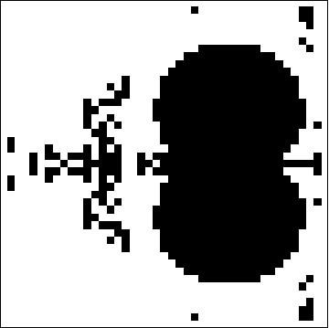
That looks like it might be interesting, possibly even fractal, behaviour but I need to increase the resolution and maybe widen the range to see what’s really going on. That’s going to take quite a bit of calculation time so I need to optimise some more.
Going Parallel
There is no point in having machines with two, four or more processor cores if you only ever use one and so it is time to see if we can get our other cores in on the act.
It turns out that this calculation is an example of a so-called embarrassingly parallel problem and so life is going to be particularly easy for us. Basically, all we need to do is to give each core its own bit of the complex plane to work on, collect the results at the end and reap the increase in speed. Here’s the full parallel version of the power tower fractal code
(*Complete Parallel version of the power tower fractal code*)

convergeQ[base_, size_] :=
 If[Length[
 Quiet[NestWhileList[N[(base^#)] &, base, Abs[#1 - #2] > 0.01 &,
 2, size, -1]]] < size, 1, 0];

LaunchKernels[];
DistributeDefinitions[convergeQ];
ParallelEvaluate[SetSystemOptions["CatchMachineUnderflow" -> False]];

towerFractParallel[xmin_, xmax_, ymin_, ymax_, step_] :=
 ArrayPlot[
 ParallelTable[
 convergeQ[x + I y, 50], {y, ymin, ymax, step}, {x, xmin, xmax, step}
, Method -> "CoarsestGrained"]]
This code is pretty similar to the single processor version so let’s focus on the parallel modifications. My convergeQ function is no different to the serial version so nothing new to talk about there. So, the first new code is
LaunchKernels[];
This launches a set of parallel Mathematica kernels. The amount that actually get launched depends on the number of cores on your machine. So, on my dual core laptop I get 2 and on my quad core desktop I get 4.
DistributeDefinitions[convergeQ];
All of those parallel kernels are completely clean in that they don’t know about my user defined convergeQ function. This line sends the definition of convergeQ to all of the freshly launched parallel kernels.
ParallelEvaluate[SetSystemOptions["CatchMachineUnderflow" -> False]];
Here we turn off Mathematica’s machine underflow safety net on all of our parallel kernels using the ParallelEvaluate function.
That’s all that is necessary to set up the parallel environment. All that remains is to change Map to ParallelMap and to add the argument Method -> “CoarsestGrained” which basically says to Mathematica ‘Each sub-calculation will take a tiny amount of time to perform so you may as well send each core lots to do at once’ (click here for a blog post of mine where this is discussed further).
That’s all it took to take this embarrassingly parallel problem from a serial calculation to a parallel one. Let’s see if it worked. The test machine for what follows contains a T5800 Intel Core 2 Duo CPU running at 2Ghz on Ubuntu (if you want to repeat these timings then I suggest you read this blog post first or you may find the parallel version going slower than the serial one). I’ve suppressed the output of the graphic since I only want to time calculation and not rendering time.
(*Serial version*)
In[3]= AbsoluteTiming[towerFract[-2, 2, -2, 2, 0.1];]
Out[3]= {0.672976, Null}

(*Parallel version*)
In[4]= AbsoluteTiming[towerFractParallel[-2, 2, -2, 2, 0.1];]
Out[4]= {0.532504, Null}

In[5]= speedup = 0.672976/0.532504
Out[5]= 1.2638
I was hoping for a bit more than a factor of 1.26 but that’s the way it goes with parallel programming sometimes. The speedup factor gets a bit higher if you increase the size of the problem though. Let’s increase the problem size by a factor of 100.
towerFractParallel[-2, 2, -2, 2, 0.01]
The above calculation took 41.99 seconds compared to 63.58 seconds for the serial version resulting in a speedup factor of around 1.5 (or about 34% depending on how you want to look at it).
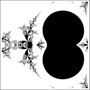
Other optimisations
I guess if I were really serious about optimising this problem then I could take advantage of the symmetry along the x axis or maybe I could utilise the fact that if one point in a convergence spiral converges then it follows that they all do. Maybe there are more intelligent ways to test for convergence or maybe I’d get a big speed increase from programming in C or F#? If anyone is interested in having a go at improving any of this and succeeds then let me know.
I’m not going to pursue any of these or any other optimisations, however, since the above exploration is what I achieved in a single train journey to work (The write-up took rather longer though). I didn’t know where I was going and I only worried about optimisation when I had to. At each step of the way the code was fast enough to ensure that I could interact with the problem at hand.
Being mostly ‘fast enough’ with minimal programming effort is one of the reasons I like playing with Mathematica when doing explorations such as this.
Treading where people have gone before
So, back to the power tower story. As I mentioned earlier, I did most of the above in a single train journey and I didn’t have access to the internet. I was quite excited that I had found a fractal from such a relatively simple system and very much felt like I had discovered something for myself. Would this lead to something that was publishable I wondered?
Sadly not!
It turns out that power towers have been thoroughly investigated and the act of forming a tower is called tetration. I learned that when a tower converges there is an analytical formula that gives what it will converge to:

Where W is the Lambert W function (click here for a cool poster for this function). I discovered that other people had already made Wolfram Demonstrations for power towers too
There is even a website called tetration.org that shows ‘my’ fractal in glorious technicolor. Nothing new under the sun eh?
Parting shots
Well, I didn’t discover anything new but I had a bit of fun along the way. Here’s the final Manipulate I came up with
Manipulate[const = p[[1]] + p[[2]] I;
 If[hz,
  ListPlot[fasttowerspiral[const, n], PlotRange -> {{-2, 2}, {-2, 2}},
    Axes -> ax,
   Epilog -> {{PointSize[Large], Red,
      Point[complexSplit[N[h[const]]]]}, {Inset[
       Framed[N[h[const]]], {-1, -1.5}]}}]
  , ListPlot[fasttowerspiral[const, n],
   PlotRange -> {{-2, 2}, {-2, 2}}, Axes -> ax]
  ]
 , {{n, 100, "Number of terms"}, 1, 500, 1, Appearance -> "Labeled"}
 , {{ax, True, "Show axis"}, {True, False}}
 , {{hz, True, "Show h(z)"}, {True, False}}
 , {{p, {0, 1.5}}, Locator}
 , Initialization :> (
   SetSystemOptions["CatchMachineUnderflow" -> False];
   complexSplit[x_] := {Re[x], Im[x]};
   fasttowerspiral[base_, size_] :=
    Quiet[Map[complexSplit,
      NestWhileList[N[(base^#)] &, base, MatchQ[#, _Complex] &, 1,
       size, -1]]];
   h[z_] := -ProductLog[-Log[z]]/Log[z];
   )
 ]
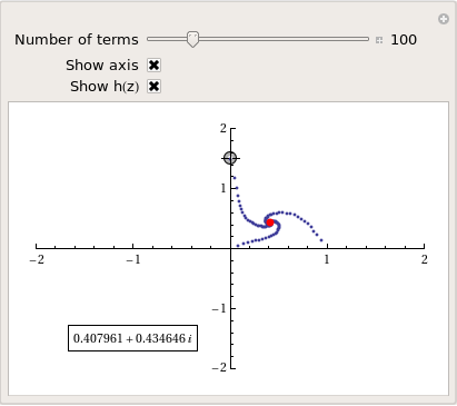
and here’s a video of a zoom into the tetration fractal that I made using spare cycles on Manchester University’s condor pool.
If you liked this blog post then you may also enjoy: