
Archive for the ‘matlab’ Category
This article is the third part of a series where I look at rewriting a particular piece of MATLAB code using various techniques. The introduction to the series is here and the introduction to the larger series of GPU articles for MATLAB is here.
Last time I used The Mathwork’s Parallel Computing Toolbox in order to modify a simple correlated asset calculation to run on my laptop’s GPU rather than its CPU. Performance was not as good as I had hoped and I never managed to get my laptop’s GPU (an NVIDIA GT555M) to beat the CPU using functions from the parallel computing toolbox. Transferring the code to a much more powerful Tesla GPU card resulted in a four times speed-up compared to the CPU in my laptop.
This time I’ll take a look at AccelerEyes’ Jacket, a third party GPU solution for MATLAB.
Attempt 1 – Make as few modifications as possible
I started off just as I did for the parallel computing toolbox GPU port; by taking the best CPU-only code from part 1 (optimised_corr2.m) and changing a load of data-types from double to gdouble in order to get the calculation to run on my laptop’s GPU using Jacket v1.8.1 and MATLAB 2010b. I also switched to using the GPU versions of various functions such as grandn instead of randn for example. Functions such as cumprod needed no modifications at all since they are nicely overloaded; if the argument to cumprod is of type double then the calculation happens on the CPU whereas if it is gdouble then it happens on the GPU.
Now, one thing that I don’t like about Jacket’s implementation is that many of the functions return single precision numbers by default. For example, if you do
a=grand(1,10)
then you end up with 10 numbers of type gsingle. To get double precision numbers you have to do
grandn(1,10,'double')
Now you may be thinking ‘what’s the big deal? – it’s just a bit of syntax so get over it’ and I guess that would be a fair comment. Supporting single precision also allows users of legacy GPUs to get in on the GPU-accelerated action which is a good thing. The problem as I see it is that almost everything else in MATLAB uses double precision numbers as the default and so it’s easy to get caught out. I would much rather see functions such as grand return double precision by default with the option to use single precision if required–just like almost every other MATLAB function out there.
The result of my ‘port’ is GPU_jacket_corr1.m
One thing to note in this version, along with all subsequent Jacket versions, is the following command that appears at the very end of the program.
gsync;
This is very important if you want to get meaningful timing results since it ensures that all GPU computations have finished before execution continues. See the Jacket documentation on gysnc and this blog post on timing Jacket code for more details.
The other thing I’ll mention is that, in this version, I do this:
Corr = [1 0.4; 0.4 1];
UpperTriangle=gdouble(chol(Corr));
instead of
Corr = gdouble([1 0.4; 0.4 1]);
UpperTriangle=chol(Corr);
In other words, I do the cholesky decomposition on the CPU and move the results to the GPU rather than doing the calculation on the GPU. This is mainly because I don’t have access to a Jacket DLA license but it’s probably the best thing to do anyway since such a small decomposition probably won’t happen any faster on the GPU.
So, how does it perform. I ran it three times with the now usual parameters of 100000 simulations done in blocks of 125 (see the CPU version for how I came to choose 125)
>> tic;GPU_jacket_corr1;toc
Elapsed time is 40.691888 seconds.
>> tic;GPU_jacket_corr1;toc
Elapsed time is 32.096796 seconds.
>> tic;GPU_jacket_corr1;toc
Elapsed time is 32.039982 seconds.
Just like the Parallel Computing Toolbox, the first run is slower because of GPU warmup overheads. Also, just like the PCT, performance stinks! It’s clearly not enough, in this case at least, to blindly throw in a few gdoubles and hope for the best. It is worth noting, however, that this case is nowhere near as bad as the 900+ seconds we saw in the similar parallel computing toolbox version.
Jacket has punished me for being stupid (or optimistic if you want to be polite to me) but not as much as the PCT did.
Attempt 2 – Convert from a script to a function
When working with the Parallel Computing Toolbox I demonstrated that a switch from a script to a function yielded some speed-up. This wasn’t the case with the Jacket version of the code. The functional version, GPU_jacket_corr2.m, showed no discernable speed improvement compared to the script.
%Warm up run performed previously
>> tic;GPU_jacket_corr2(100000,125);toc
Elapsed time is 32.230638 seconds.
>> tic;GPU_jacket_corr2(100000,125);toc
Elapsed time is 32.179734 seconds.
>> tic;GPU_jacket_corr2(100000,125);toc
Elapsed time is 32.114864 seconds.
Attempt 3 – One big matrix multiply!
The original version of this calculation performs thousands of very small matrix multiplications and last time we saw that switching to a single, large matrix multiplication brought significant speed improvements on the GPU. Modifying the code to do this with Jacket is a very similar process to doing it for the PCT so I’ll omit the details and just present the code, GPU_jacket_corr3.m
%Warm up runs performed previously
>> tic;GPU_jacket_corr3(100000,125);toc
Elapsed time is 2.041111 seconds.
>> tic;GPU_jacket_corr3(100000,125);toc
Elapsed time is 2.025450 seconds.
>> tic;GPU_jacket_corr3(100000,125);toc
Elapsed time is 2.032390 seconds.
Now that’s more like it! Finally we have a GPU version that runs faster than the CPU on my laptop. We can do better, however, since the block size of 125 was chosen especially for my CPU. With this Jacket version bigger is better and we get much more speed-up by switching to a block size of 25000 (I run out of memory on the GPU if I try even bigger block sizes).
%Warm up runs performed previously
>> tic;GPU_jacket_corr3(100000,25000);toc
Elapsed time is 0.749945 seconds.
>> tic;GPU_jacket_corr3(100000,25000);toc
Elapsed time is 0.749333 seconds.
>> tic;GPU_jacket_corr3(100000,25000);toc
Elapsed time is 0.749556 seconds.
Now this is exciting! My laptop GPU with Jacket 1.8.1 is faster than a high-end Tesla card using the parallel computing toolbox for this calculation. My excitement was short lived, however, when I looked at the resulting distribution. The random number generator in Jacket 1.8.1 gave a completely different distribution when compared to generators from other sources (I tried two CPU generators from The Mathworks and one from The Numerical Algorithms Group). The only difference in the code that generated the results below is the random number generator used.
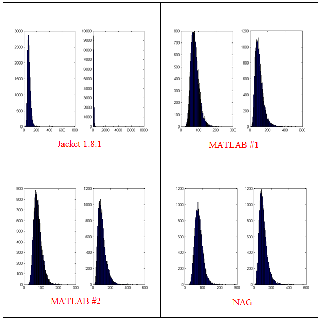
- The results shown in these plots were for only 20,000 simulations rather than the 100,000 I’ve been using elsewhere in this post. I found this bug in the development stage of these posts where I was using a smaller number of simulations.
- Jacket 1.8.1 is using Jackets old grandn function with the ‘double’ option set
- MATLAB #1 is using MATLAB’s randn using the Comb Recursive algorithm on the CPU
- MATLAB #2 is using MATLAB’s randn using the default Mersenne Twister on the CPU
- NAG is using a Wichman-Hill generator
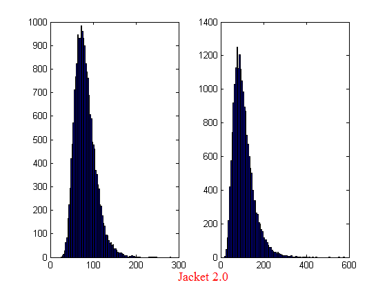
I sent my code to AccelerEye’s customer support who confirmed that this seemed to be a bug in their random number generator (an in-house Mersenne Twister implementation). Less than a week later they offered me a new preview of Jacket from their Nightly builds where the old RNG had been replaced with the Mersenne Twister implementation produced by NVidia and I’m happy to confirm that not only does this fix the results for my code but it goes even faster! Superb customer service!
This new RNG is now the default in version 2.0 of Jacket. Here’s the distribution I get for 20,000 simulations (to stay in line with the plots shown above).
Switching back to 100,000 simulations to stay in line with all of the other benchmarks in this series gives the following times on my laptop’s GPU
%Warm up runs performed previously
>> tic;prices=GPU_jacket_corr3(100000,25000);toc
Elapsed time is 0.696891 seconds.
>> tic;prices=GPU_jacket_corr3(100000,25000);toc
Elapsed time is 0.697596 seconds.
>> tic;prices=GPU_jacket_corr3(100000,25000);toc
Elapsed time is 0.697312 seconds.
This is almost 5 times faster than the 3.42 seconds managed by the best CPU version from part 1. I sent my code to AccelerEyes and asked them to run it on a more powerful GPU, a Tesla C2075, and these are the results they sent back
Elapsed time is 5.246249 seconds. %warm up run
Elapsed time is 0.158165 seconds.
Elapsed time is 0.156529 seconds.
Elapsed time is 0.156522 seconds.
Elapsed time is 0.156501 seconds.
So, the Tesla is 4.45 times faster than my laptop’s GPU for this application and a very useful 21.85 times faster than my laptop’s CPU.
Results Summary
- Best CPU Result on laptop (i7-2630GM)with pure MATLAB code – 3.42 seconds
- Best GPU Result with PCT on laptop (GT555M) – 4.04 seconds
- Best GPU Result with PCT on Tesla M2070 – 0.85 seconds
- Best GPU Result with Jacket on laptop (GT555M) – 0.7 seconds
- Best GPU Result with Jacket on Tesla M2075 – 0.16 seconds
Test System Specification
- Laptop model: Dell XPS L702X
- CPU:Intel Core i7-2630QM @2Ghz software overclockable to 2.9Ghz. 4 physical cores but total 8 virtual cores due to Hyperthreading.
- GPU:GeForce GT 555M with 144 CUDA Cores. Graphics clock: 590Mhz. Processor Clock:1180 Mhz. 3072 Mb DDR3 Memeory
- RAM: 8 Gb
- OS: Windows 7 Home Premium 64 bit.
- MATLAB: 2011b
Acknowledgements
Thanks to Yong Woong Lee of the Manchester Business School as well as various employees at AccelerEyes for useful discussions and advice. Any mistakes that remain are all my own.
This article is the second part of a series where I look at rewriting a particular piece of MATLAB code using various techniques. The introduction to the series is here and the introduction to the larger series of GPU articles for MATLAB on WalkingRandomly is here.
Attempt 1 – Make as few modifications as possible
I took my best CPU-only code from last time (optimised_corr2.m) and changed a load of data-types from double to gpuArray in order to get the calculation to run on my laptop’s GPU using the parallel computing toolbox in MATLAB 2010b. I also switched to using the GPU versions of various functions such as parallel.gpu.GPUArray.randn instead of randn for example. Functions such as cumprod needed no modifications at all since they are nicely overloaded; if the argument to cumprod is of type double then the calculation happens on the CPU whereas if it is gpuArray then it happens on the GPU.
The above work took about a minute to do which isn’t bad for a CUDA ‘porting’ effort! The result, which I’ve called GPU_PCT_corr1.m is available for you to download and try out.
How about performance? Let’s do a quick tic and toc using my laptop’s NVIDIA GT 555M GPU.
>> tic;GPU_PCT_corr1;toc
Elapsed time is 950.573743 seconds.
The CPU version of this code took only 3.42 seconds which means that this GPU version is over 277 times slower! Something has gone horribly, horribly wrong!
Attempt 2 – Switch from script to function
In general functions should be faster than scripts in MATLAB because more automatic optimisations are performed on functions. I didn’t see any difference in the CPU version of this code (see optimised_corr3.m from part 1 for a CPU function version) and so left it as a script (partly so I had an excuse to discuss it here if I am honest). This GPU-version, however, benefits noticeably from conversion to a function. To do this, add the following line to the top of GPU_PCT_corr1.m
function [SimulPrices] = GPU_PTC_corr2( n,sub_size)
Next, you need to delete the following two lines
n=100000;                       %Number of simulations
sub_size = 125;
Finally, add the following to the end of our new function
end
That’s pretty much all I did to get GPU_PCT_corr2.m. Let’s see how that performs using the same parameters as our script (100,000 simulations in blocks of 125). I used script_vs_func.m to run both twice after a quick warm-up iteration and the results were:
Warm up
Elapsed time is 1.195806 seconds.
Main event
script
Elapsed time is 950.399920 seconds.
function
Elapsed time is 938.238956 seconds.
script
Elapsed time is 959.420186 seconds.
function
Elapsed time is 939.716443 seconds.
So, switching to a function has saved us a few seconds but performance is still very bad!
Attempt 3 – One big matrix multiply!
So far all I have done is take a program that works OK on a CPU, and run it exactly as-is on the GPU in the hope that something magical would happen to make it go faster. Of course, GPUs and CPUs are very different beasts with differing sets of strengths and weaknesses so it is rather naive to think that this might actually work. What we need to do is to play to the GPUs strengths more and the way to do this is to focus on this piece of code.
for i=1:sub_size
     CorrWiener(:,:,i)=parallel.gpu.GPUArray.randn(T-1,2)*UpperTriangle;
end
Here, we are performing lots of small matrix multiplications and, as mentioned in part 1, we might hope to get better performance by performing just one large matrix multiplication instead. To do this we can change the above code to
%Generate correlated random numbers
%using one big multiplication
randoms = parallel.gpu.GPUArray.randn(sub_size*(T-1),2);
CorrWiener = randoms*UpperTriangle;
CorrWiener = reshape(CorrWiener,(T-1),sub_size,2);
%CorrWiener = permute(CorrWiener,[1 3 2]); %Can't do this on the GPU in 2011b or below

%poor man's permute since GPU permute if not available in 2011b
CorrWiener_final = parallel.gpu.GPUArray.zeros(T-1,2,sub_size);
for s = 1:2
    CorrWiener_final(:, s, :) = CorrWiener(:, :, s);
end
The reshape and permute are necessary to get the matrix in the form needed later on. Sadly, MATLAB 2011b doesn’t support permute on GPUArrays and so I had to use the ‘poor mans permute’ instead.
The result of the above is contained in GPU_PCT_corr3.m so let’s see how that does in a fresh instance of MATLAB.
>> tic;GPU_PCT_corr3(100000,125);toc
Elapsed time is 16.666352 seconds.
>> tic;GPU_PCT_corr3(100000,125);toc
Elapsed time is 8.725997 seconds.
>> tic;GPU_PCT_corr3(100000,125);toc
Elapsed time is 8.778124 seconds.
The first thing to note is that performance is MUCH better so we appear to be on the right track. The next thing to note is that the first evaluation is much slower than all subsequent ones. This is totally expected and is due to various start-up overheads.
Recall that 125 in the above function calls refers to the block size of our monte-carlo simulation. We are doing 100,000 simulations in blocks of 125– a number chosen because I determined empirically that this was the best choice on my CPU. It turns out we are better off using much larger block sizes on the GPU:
>> tic;GPU_PCT_corr3(100000,250);toc
Elapsed time is 6.052939 seconds.
>> tic;GPU_PCT_corr3(100000,500);toc
Elapsed time is 4.916741 seconds.
>> tic;GPU_PCT_corr3(100000,1000);toc
Elapsed time is 4.404133 seconds.
>> tic;GPU_PCT_corr3(100000,2000);toc
Elapsed time is 4.223403 seconds.
>> tic;GPU_PCT_corr3(100000,5000);toc
Elapsed time is 4.069734 seconds.
>> tic;GPU_PCT_corr3(100000,10000);toc
Elapsed time is 4.039446 seconds.
>> tic;GPU_PCT_corr3(100000,20000);toc
Elapsed time is 4.068248 seconds.
>> tic;GPU_PCT_corr3(100000,25000);toc
Elapsed time is 4.099588 seconds.
The above, rather crude, test suggests that block sizes of 10,000 are the best choice on my laptop’s GPU. Sadly, however, it’s STILL slower than the 3.42 seconds I managed on the i7 CPU and represents the best I’ve managed using pure MATLAB code. The profiler tells me that the vast majority of the GPU execution time is spent in the cumprod line and in random number generation (over 40% each).
Trying a better GPU
Of course now that I have code that runs on a GPU I could just throw it at a better GPU and see how that does. I have access to MATLAB 2011b on a Tesla M2070 hooked up to a Linux machine so I ran the code on that. I tried various block sizes and the best time was 0.8489 seconds with the call GPU_PCT_corr3(100000,20000) which is just over 4 times faster than my laptop’s CPU.
Ask the Audience
Can you do better using just the GPU functionality provided in the Parallel Computing Toolbox (so no bespoke CUDA kernels or Jacket just yet)? I’ll be looking at how AccelerEyes’ Jacket myself in the next post.
Results so far
- Best CPU Result on laptop (i7-2630GM)with pure MATLAB code – 3.42 seconds
- Best GPU Result with PCT on laptop (GT555M) – 4.04 seconds
- Best GPU Result with PCT on Tesla M2070 – 0.85 seconds
Test System Specification
- Laptop model: Dell XPS L702X
- CPU: Intel Core i7-2630QM @2Ghz software overclockable to 2.9Ghz. 4 physical cores but total 8 virtual cores due to Hyperthreading.
- GPU: GeForce GT 555M with 144 CUDA Cores. Graphics clock: 590Mhz. Processor Clock:1180 Mhz. 3072 Mb DDR3 Memeory
- RAM: 8 Gb
- OS: Windows 7 Home Premium 64 bit.
- MATLAB: 2011b
Acknowledgements
Thanks to Yong Woong Lee of the Manchester Business School as well as various employees at The Mathworks for useful discussions and advice. Any mistakes that remain are all my own :)
Recently, I’ve been working with members of The Manchester Business School to help optimise their MATLAB code. We’ve had some great successes using techniques such as vectorisation, mex files and The NAG Toolbox for MATLAB (among others) combined with the raw computational power of Manchester’s Condor Pool (which I help run along with providing applications support).
A couple of months ago, I had the idea of taking a standard calculation in computational finance and seeing how fast I could make it run on MATLAB using various techniques. I’d then write these up and publish here for comment.
So, I asked one of my collaborators, Yong Woong Lee, a doctoral researcher in the Manchester Business School, if he could furnish me with a very simple piece computational finance code. I asked for something that was written to make it easy to see the underlying mathematics rather than for speed and he duly obliged with several great examples. I took one of these examples and stripped it down even further to its very bare bones. In doing so I may have made his example close to useless from a computational finance point of view but it gave me something nice and simple to play with.
What I ended up with was a simple piece of code that uses monte carlo techniques to find the distribution of two correlated assets: original_corr.m
%ORIGINAL_CORR - The original, unoptimised code that simulates two correlated assets

%% Correlated asset information
CurrentPrice = [78 102];       %Initial Prices of the two stocks
Corr = [1 0.4; 0.4 1];         %Correlation Matrix
T = 500;                       %Number of days to simulate = 2years = 500days
n = 100000;                    %Number of simulations
dt = 1/250;                    %Time step (1year = 250days)
Div=[0.01 0.01];               %Dividend
Vol=[0.2 0.3];                 %Volatility

%%Market Information
r = 0.03;                      %Risk-free rate

%% Define storages
SimulPriceA=zeros(T,n);    %Simulated Price of Asset A
SimulPriceA(1,:)=CurrentPrice(1);
SimulPriceB=zeros(T,n);    %Simulated Price of Asset B
SimulPriceB(1,:)=CurrentPrice(2);

%% Generating the paths of stock prices by Geometric Brownian Motion
UpperTriangle=chol(Corr);    %UpperTriangle Matrix by Cholesky decomposition

for i=1:n
   Wiener=randn(T-1,2);
   CorrWiener=Wiener*UpperTriangle;
   for j=2:T
      SimulPriceA(j,i)=SimulPriceA(j-1,i)*exp((r-Div(1)-Vol(1)^2/2)*dt+Vol(1)*sqrt(dt)*CorrWiener(j-1,1));
      SimulPriceB(j,i)=SimulPriceB(j-1,i)*exp((r-Div(2)-Vol(2)^2/2)*dt+Vol(2)*sqrt(dt)*CorrWiener(j-1,2));
   end
end

%% Plot the distribution of final prices
% Comment this section out if doing timings
% subplot(1,2,1);hist(SimulPriceA(end,:),100);
% subplot(1,2,2);hist(SimulPriceB(end,:),100);
On my laptop, this code takes 10.82 seconds to run on average. If you comment out the final two lines then it’ll take a little longer and will produce a histogram of the distribution of final prices.
I’m going to take this code and modify it in various ways to see how different techniques and technologies can make it run more quickly. Here is a list of everything I have done so far.
- Standard vectorisation (This article)
- Running on a GPU using the Parallel Computing Toolbox
- Running on a GPU using Jacket from AccelerEyes
Vectorisation – removing loops to make code go faster
Now, the most obvious optimisation that we can do with code like this is to use vectorisation to get rid of that double loop. The cumprod command is the key to doing this and the resulting code looks as follows: optimised_corr1.m
%OPTIMISED_CORR1 - A pure-MATLAB optimised code that simulates two correlated assets

%% Correlated asset information
CurrentPrice = [78 102];       %Initial Prices of the two stocks
Corr = [1 0.4; 0.4 1];         %Correlation Matrix
T = 500;                       %Number of days to simulate = 2years = 500days
Div=[0.01 0.01];               %Dividend
Vol=[0.2 0.3];                 %Volatility

%% Market Information
r = 0.03;                      %Risk-free rate

%% Simulation parameters
n=100000;                       %Number of simulation
dt=1/250;                       %Time step (1year = 250days)

%% Define storages
SimulPrices=repmat(CurrentPrice,n,1);
CorrWiener = zeros(T-1,2,n);

%% Generating the paths of stock prices by Geometric Brownian Motion
UpperTriangle=chol(Corr);    %UpperTriangle Matrix by Cholesky decomposition

for i=1:n
     CorrWiener(:,:,i)=randn(T-1,2)*UpperTriangle;
end
Volr = repmat(Vol,[T-1,1,n]);
Divr = repmat(Div,[T-1,1,n]);

%% do simulation
sim = cumprod(exp((r-Divr-Volr.^2./2).*dt+Volr.*sqrt(dt).*CorrWiener));
%get just the final prices
SimulPrices = SimulPrices.*reshape(sim(end,:,:),2,n)';

%% Plot the distribution of final prices
% Comment this section out if doing timings
%subplot(1,2,1);hist(SimulPrices(:,1),100);
%subplot(1,2,2);hist(SimulPrices(:,2),100);
This code takes an average of 4.19 seconds to run on my laptop giving us a factor of 2.58 times speed up over the original. This improvement in speed is not without its cost, however, and the price we have to pay is memory. Let’s take a look at the amount of memory used by MATLAB after running these two versions. First, the original
>> clear all
>> memory
Maximum possible array:              13344 MB (1.399e+010 bytes) *
Memory available for all arrays:     13344 MB (1.399e+010 bytes) *
Memory used by MATLAB:                 553 MB (5.800e+008 bytes)
Physical Memory (RAM):                8106 MB (8.500e+009 bytes)

*  Limited by System Memory (physical + swap file) available.
>> original_corr
>> memory
Maximum possible array:              12579 MB (1.319e+010 bytes) *
Memory available for all arrays:     12579 MB (1.319e+010 bytes) *
Memory used by MATLAB:                1315 MB (1.379e+009 bytes)
Physical Memory (RAM):                8106 MB (8.500e+009 bytes)

*  Limited by System Memory (physical + swap file) available.
Now for the vectorised version
>> %now I clear the workspace and check that all memory has been recovered%
>> clear all
>> memory
Maximum possible array:              13343 MB (1.399e+010 bytes) *
Memory available for all arrays:     13343 MB (1.399e+010 bytes) *
Memory used by MATLAB:                 555 MB (5.818e+008 bytes)
Physical Memory (RAM):                8106 MB (8.500e+009 bytes)

*  Limited by System Memory (physical + swap file) available.
>> optimised_corr1
>> memory
Maximum possible array:              10297 MB (1.080e+010 bytes) *
Memory available for all arrays:     10297 MB (1.080e+010 bytes) *
Memory used by MATLAB:                3596 MB (3.770e+009 bytes)
Physical Memory (RAM):                8106 MB (8.500e+009 bytes)

*  Limited by System Memory (physical + swap file) available.
So, the original version used around 762Mb of RAM whereas the vectorised version used 3041Mb. If you don’t have enough memory then you may find that the vectorised version runs very slowly indeed!
Adding a loop to the vectorised code to make it go even faster!
Simple vectorisation improvements such as the one above are sometimes so effective that it can lead MATLAB programmers to have a pathological fear of loops. This fear is becoming increasingly unjustified thanks to the steady improvements in MATLAB’s Just In Time (JIT) compiler. Discussing the details of MATLAB’s JIT is beyond the scope of these articles but the practical upshot is that you don’t need to be as frightened of loops as you used to.
In fact, it turns out that once you have finished vectorising your code, you may be able to make it go even faster by putting a loop back in (not necessarily thanks to the JIT though)! The following code takes an average of 3.42 seconds on my laptop bringing the total speed-up to a factor of 3.16 compared to the original. The only difference is that I have added a loop over the variable ii to split up the cumprod calculation over groups of 125 at a time.
I have a confession: I have no real idea why this modification causes the code to go noticeably faster. I do know that it uses a lot less memory; using the memory command, as I did above, I determined that it uses around 10Mb compared to 3041Mb of the original vectorised version. You may be wondering why I set sub_size to be 125 since I could have chosen any divisor of 100000. Well, I tried them all and it turned out that 125 was slightly faster than any other on my machine. Maybe we are seeing some sort of CPU cache effect? I just don’t know: optimised_corr2.m
%OPTIMISED_CORR2 - A pure-MATLAB optimised code that simulates two correlated assets
%% Correlated asset information
CurrentPrice = [78 102];       %Initial Prices of the two stocks
Corr = [1 0.4; 0.4 1];         %Correlation Matrix
T = 500;                       %Number of days to simulate = 2years = 500days
Div=[0.01 0.01];               %Dividend
Vol=[0.2 0.3];                 %Volatility

%% Market Information
r = 0.03;                      %Risk-free rate

%% Simulation parameters
n=100000;                       %Number of simulation
sub_size = 125;
dt=1/250;                       %Time step (1year = 250days)

%% Define storages
SimulPrices=repmat(CurrentPrice,n,1);
CorrWiener = zeros(T-1,2,sub_size);

%% Generating the paths of stock prices by Geometric Brownian Motion
UpperTriangle=chol(Corr);    %UpperTriangle Matrix by Cholesky decomposition
Volr = repmat(Vol,[T-1,1,sub_size]);
Divr = repmat(Div,[T-1,1,sub_size]);

for ii = 1:sub_size:n
   for i=1:sub_size
        CorrWiener(:,:,i)=randn(T-1,2)*UpperTriangle;
   end

   %% do simulation
   sim = cumprod(exp((r-Divr-Volr.^2./2).*dt+Volr.*sqrt(dt).*CorrWiener));
   %get just the final prices
   SimulPrices(ii:ii+sub_size-1,:) = SimulPrices(ii:ii+sub_size-1,:).*reshape(sim(end,:,:),2,sub_size)';
end
%% Plot the distribution of final prices
% Comment this section out if doing timings
%subplot(1,2,1);hist(SimulPrices(:,1),100);
%subplot(1,2,2);hist(SimulPrices(:,2),100);
Some things that might have worked (but didn’t)
- In general, functions are faster than scripts in MATLAB because MATLAB employs more aggressive optimisation techniques for functions. In this case, however, it didn’t make any noticeable difference on my machine. Try it out for yourself with optimised_corr3.m
- When generating the correlated random numbers, the above code performs lots of small matrix multiplications:
   for i=1:sub_size
        CorrWiener(:,:,i)=randn(T-1,2)*UpperTriangle;
   end
It is often the case that you can get more flops out of a system by doing a single large matrix-matrix multiply than lots of little ones. So, we could do this instead:
%Generate correlated random numbers
%using one big multiplication
randoms = randn(sub_size*(T-1),2);
CorrWiener = randoms*UpperTriangle;
CorrWiener = reshape(CorrWiener,(T-1),sub_size,2);
CorrWiener = permute(CorrWiener,[1 3 2]);
Sadly, however, any gains that we might have made by doing a single matrix-matrix multiply are lost when the resulting matrix is reshaped and permuted into the form needed for the rest of the code (on my machine at least). Feel free to try for yourself using optimised_corr4.m – the input argument of which determines the sub_size.
Ask the audience
Can you do better using nothing but pure matlab (i.e. no mex, parallel computing toolbox, GPUs or other such trickery…they are for later articles)? If so then feel free to contact me and let me know.
Acknowledgements
Thanks to Yong Woong Lee of the Manchester Business School as well as various employees at The Mathworks for useful discussions and advice. Any mistakes that remain are all my own :)
License
All code listed in this article is licensed under the 3-clause BSD license.
The test laptop
- Laptop model: Dell XPS L702X
- CPU: Intel Core i7-2630QM @2Ghz software overclockable to 2.9Ghz. 4 physical cores but total 8 virtual cores due to Hyperthreading.
- GPU: GeForce GT 555M with 144 CUDA Cores. Graphics clock: 590Mhz. Processor Clock:1180 Mhz. 3072 Mb DDR3 Memeory
- RAM: 8 Gb
- OS: Windows 7 Home Premium 64 bit.
- MATLAB: 2011b
Next Time
In the second part of this series I look at how to run this code on the GPU using The Mathworks’ Parallel Computing Toolbox.
My attention was recently drawn to a Google+ post by JerWei Zhang where he evaluates 2^3^4 in various packages and notes that they don’t always agree. For example, in MATLAB 2010a we have 2^3^4 = 4096 which is equivalent to putting (2^3)^4 whereas Mathematica 8 gives 2^3^4 = 2417851639229258349412352 which is the same as putting 2^(3^4). JerWei’s post gives many more examples including Excel, Python and Google and the result is always one of these two (although to varying degrees of precision).
What surprised me was the fact that they disagreed at all since I thought that the operator precendence rules were an agreed standard across all software packages. In this case I’d always use brackets since _I_ am not sure what the correct interpretation of 2^3^4 should be but I would have taken it for granted that there is a standard somewhere and that all of the big hitters in the numerical world would adhere to it.
Looks like I was wrong!
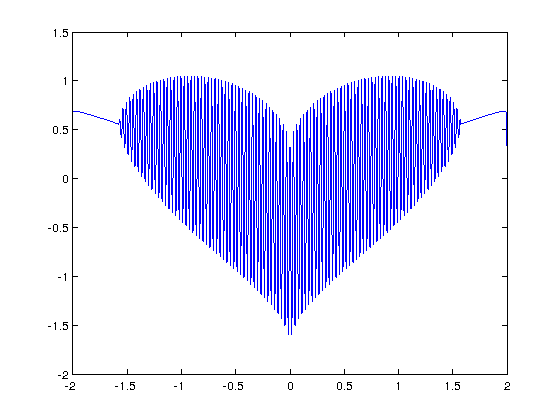
I’ve seen several equations that plot a heart shape over the years but a recent google+ post by Lionel Favre introduced me to a new one. I liked it so much that I didn’t want to wait until Valentine’s day to share it. In Mathematica:
Plot[Sqrt[Cos[x]]*Cos[200*x] + Sqrt[Abs[x]] - 0.7*(4 - x*x)^0.01, {x, -2, 2}]
and in MATLAB:
>> x=[-2:.001:2];
>> y=(sqrt(cos(x)).*cos(200*x)+sqrt(abs(x))-0.7).*(4-x.*x).^0.01;
>> plot(x,y)
Warning: Imaginary parts of complex X and/or Y arguments ignored
The result from the MATLAB version is shown below
Update
Rene Grothmann has looked at this equation in a little more depth and plotted it using Euler.
Similar posts
Modern CPUs are capable of parallel processing at multiple levels with the most obvious being the fact that a typical CPU contains multiple processor cores. My laptop, for example, contains a quad-core Intel Sandy Bridge i7 processor and so has 4 processor cores. You may be forgiven for thinking that, with 4 cores, my laptop can do up to 4 things simultaneously but life isn’t quite that simple.
The first complication is hyper-threading where each physical core appears to the operating system as two or more virtual cores. For example, the processor in my laptop is capable of using hyper-threading and so I have access to up to 8 virtual cores! I have heard stories where unscrupulous sales people have passed off a 4 core CPU with hyperthreading as being as good as an 8 core CPU…. after all, if you fire up the Windows Task Manager you can see 8 cores and so there you have it! However, this is very far from the truth since what you really have is 4 real cores with 4 brain damaged cousins. Sometimes the brain damaged cousins can do something useful but they are no substitute for physical cores. There is a great explanation of this technology at makeuseof.com.
The second complication is the fact that each physical processor core contains a SIMD (Single Instruction Multiple Data) lane of a certain width. SIMD lanes, aka SIMD units or vector units, can process several numbers simultaneously with a single instruction rather than only one a time. The 256-bit wide SIMD lanes on my laptop’s processor, for example, can operate on up to 8 single (or 4 double) precision numbers per instruction. Since each physical core has its own SIMD lane this means that a 4 core processor could theoretically operate on up to 32 single precision (or 16 double precision) numbers per clock cycle!
So, all we need now is a way of programming for these SIMD lanes!
Intel’s SPMD Program Compiler, ispc, is a free product that allows programmers to take direct advantage of the SIMD lanes in modern CPUS using a C-like syntax. The speed-ups compared to single-threaded code can be impressive with Intel reporting up to 32 times speed-up (on an i7 quad-core) for a single precision Black-Scholes option pricing routine for example.
Using ispc on MATLAB
Since ispc routines are callable from C, it stands to reason that we’ll be able to call them from MATLAB using mex. To demonstrate this, I thought that I’d write a sqrt function that works faster than MATLAB’s built-in version. This is a tall order since the sqrt function is pretty fast and is already multi-threaded. Taking the square root of 200 million random numbers doesn’t take very long in MATLAB:
>> x=rand(1,200000000)*10;
>> tic;y=sqrt(x);toc
Elapsed time is 0.666847 seconds.
This might not be the most useful example in the world but I wanted to focus on how to get ispc to work from within MATLAB rather than worrying about the details of a more interesting example.
Step 1 – A reference single-threaded mex file
Before getting all fancy, let’s write a nice, straightforward single-threaded mex file in C and see how fast that goes.
#include <math.h>
#include "mex.h"

void mexFunction( int nlhs, mxArray *plhs[], int nrhs, const mxArray *prhs[] )
{
    double *in,*out;
    int rows,cols,num_elements,i;

    /*Get pointers to input matrix*/
    in = mxGetPr(prhs[0]);
    /*Get rows and columns of input matrix*/
    rows = mxGetM(prhs[0]);
    cols = mxGetN(prhs[0]);
    num_elements = rows*cols;

    /* Create output matrix */
    plhs[0] = mxCreateDoubleMatrix(rows, cols, mxREAL);
    /* Assign pointer to the output */
    out = mxGetPr(plhs[0]);

    for(i=0; i<num_elements; i++)
    {
        out[i] = sqrt(in[i]);
    }
}
Save the above to a text file called sqrt_mex.c and compile using the following command in MATLAB
mex sqrt_mex.c
Let’s check out its speed:
>> x=rand(1,200000000)*10;
>> tic;y=sqrt_mex(x);toc
Elapsed time is 1.993684 seconds.
Well, it works but it’s quite a but slower than the built-in MATLAB function so we still have some work to do.
Step 2 – Using the SIMD lane on one core via ispc
Using ispc is a two step process. First of all you need the .ispc program
export void ispc_sqrt(uniform double vin[], uniform double vout[],
                   uniform int count) {
    foreach (index = 0 ... count) {
        vout[index] = sqrt(vin[index]);
    }
}
Save this to a file called ispc_sqrt.ispc and compile it at the Bash prompt using
ispc -O2 ispc_sqrt.ispc -o ispc_sqrt.o -h ispc_sqrt.h --pic
This creates an object file, ispc_sqrt.o, and a header file, ispc_sqrt.h. Now create the mex file in MATLAB
#include <math.h>
#include "mex.h"
#include "ispc_sqrt.h"

void mexFunction( int nlhs, mxArray *plhs[], int nrhs, const mxArray *prhs[] )
{
    double *in,*out;
    int rows,cols,num_elements,i;

    /*Get pointers to input matrix*/
    in = mxGetPr(prhs[0]);
    /*Get rows and columns of input matrix*/
    rows = mxGetM(prhs[0]);
    cols = mxGetN(prhs[0]);
    num_elements = rows*cols;

    /* Create output matrix */
    plhs[0] = mxCreateDoubleMatrix(rows, cols, mxREAL);
    /* Assign pointer to the output */
    out = mxGetPr(plhs[0]);

    ispc::ispc_sqrt(in,out,num_elements);
}
Call this ispc_sqrt_mex.cpp and compile in MATLAB with the command
mex ispc_sqrt_mex.cpp ispc_sqrt.o
Let’s see how that does for speed:
>> tic;y=ispc_sqrt_mex(x);toc
Elapsed time is 1.379214 seconds.
So, we’ve improved on the single-threaded mex file a bit (1.37 instead of 2 seconds) but it’s still not enough to beat the MATLAB built-in. To do that, we are going to have to use the SIMD lanes on all 4 cores simultaneously.
Step 3 – A reference multi-threaded mex file using OpenMP
Let’s step away from ispc for a while and see how we do with something we’ve seen before– a mex file using OpenMP (see here and here for previous articles on this topic).
#include <math.h>
#include "mex.h"
#include <omp.h>

void do_calculation(double in[],double out[],int num_elements)
{
    int i;

#pragma omp parallel for shared(in,out,num_elements)
    for(i=0; i<num_elements; i++){
          out[i] = sqrt(in[i]);
         }
}

void mexFunction( int nlhs, mxArray *plhs[], int nrhs, const mxArray *prhs[] )
{
    double *in,*out;
    int rows,cols,num_elements,i;

    /*Get pointers to input matrix*/
    in = mxGetPr(prhs[0]);
    /*Get rows and columns of input matrix*/
    rows = mxGetM(prhs[0]);
    cols = mxGetN(prhs[0]);
    num_elements = rows*cols;

    /* Create output matrix */
    plhs[0] = mxCreateDoubleMatrix(rows, cols, mxREAL);
    /* Assign pointer to the output */
    out = mxGetPr(plhs[0]);

    do_calculation(in,out,num_elements);
}
Save this to a text file called openmp_sqrt_mex.c and compile in MATLAB by doing
mex openmp_sqrt_mex.c CFLAGS="\$CFLAGS -fopenmp" LDFLAGS="\$LDFLAGS -fopenmp"
Let’s see how that does (OMP_NUM_THREADS has been set to 4):
>> tic;y=openmp_sqrt_mex(x);toc
Elapsed time is 0.641203 seconds.
That’s very similar to the MATLAB built-in and I suspect that The Mathworks have implemented their sqrt function in a very similar manner. Theirs will have error checking, complex number handling and what-not but it probably comes down to a for-loop that’s been parallelized using Open-MP.
Step 4 – Using the SIMD lanes on all cores via ispc
To get a ispc program to run on all of my processors cores simultaneously, I need to break the calculation down into a series of tasks. The .ispc file is as follows
task void
ispc_sqrt_block(uniform double vin[], uniform double vout[],
                   uniform int block_size,uniform int num_elems){
    uniform int index_start = taskIndex * block_size;
    uniform int index_end = min((taskIndex+1) * block_size, (unsigned int)num_elems);

    foreach (yi = index_start ... index_end) {
        vout[yi] = sqrt(vin[yi]);
    }
}

export void
ispc_sqrt_task(uniform double vin[], uniform double vout[],
                   uniform int block_size,uniform int num_elems,uniform int num_tasks)
{

    launch[num_tasks] < ispc_sqrt_block(vin, vout, block_size, num_elems) >;
}
Compile this by doing the following at the Bash prompt
ispc -O2 ispc_sqrt_task.ispc -o ispc_sqrt_task.o -h ispc_sqrt_task.h --pic
We’ll need to make use of a task scheduling system. The ispc documentation suggests that you could use the scheduler in Intel’s Threading Building Blocks or Microsoft’s Concurrency Runtime but a basic scheduler is provided with ispc in the form of tasksys.cpp (I’ve also included it in the .tar.gz file in the downloads section at the end of this post), We’ll need to compile this too so do the following at the Bash prompt
g++ tasksys.cpp -O3 -Wall -m64 -c -o tasksys.o -fPIC
Finally, we write the mex file
#include <math.h>
#include "mex.h"
#include "ispc_sqrt_task.h"

void mexFunction( int nlhs, mxArray *plhs[], int nrhs, const mxArray *prhs[] )
{
    double *in,*out;
    int rows,cols,i;

    unsigned int num_elements;
    unsigned int block_size;
    unsigned int num_tasks;

    /*Get pointers to input matrix*/
    in = mxGetPr(prhs[0]);
    /*Get rows and columns of input matrix*/
    rows = mxGetM(prhs[0]);
    cols = mxGetN(prhs[0]);
    num_elements = rows*cols;

    /* Create output matrix */
    plhs[0] = mxCreateDoubleMatrix(rows, cols, mxREAL);
    /* Assign pointer to the output */
    out = mxGetPr(plhs[0]);

    block_size = 1000000;
    num_tasks = num_elements/block_size;

    ispc::ispc_sqrt_task(in,out,block_size,num_elements,num_tasks);

}
In the above, the input array is divided into tasks where each task takes care of 1 million elements. Our 200 million element test array will, therefore, be split into 200 tasks– many more than I have processor cores. I’ll let the task scheduler worry about how to schedule these tasks efficiently across the cores in my machine. Compile this in MATLAB by doing
mex ispc_sqrt_task_mex.cpp ispc_sqrt_task.o tasksys.o
Now for crunch time:
>> x=rand(1,200000000)*10;
>> tic;ys=sqrt(x);toc   %MATLAB's built-in
Elapsed time is 0.670766 seconds.
>> tic;y=ispc_sqrt_task_mex(x);toc  %my version using ispc
Elapsed time is 0.393870 seconds.
There we have it! A version of the sqrt function that works faster than MATLAB’s own by virtue of the fact that I am now making full use of the SIMD lanes in my laptop’s Sandy Bridge i7 processor thanks to ispc.
Although this example isn’t very useful as it stands, I hope that it shows that using the ispc compiler from within MATLAB isn’t as hard as you might think and is yet another tool in the arsenal of weaponry that can be used to make MATLAB faster.
Final Timings, downloads and links
- Single threaded: 2.01 seconds
- Single threaded with ispc: 1.37 seconds
- MATLAB built-in: 0.67 seconds
- Multi-threaded with OpenMP (OMP_NUM_THREADS=4): 0.64 seconds
- Multi-threaded with OpenMP and hyper-threading (OMP_NUM_THREADS=8): 0.55 seconds
- Task-based multicore with ispc: 0.39 seconds
Finally, here’s some links and downloads
System Specs
- MATLAB 2011b running on 64 bit linux
- gcc 4.6.1
- ispc version 1.1.1
- Intel Core i7-2630QM with 8Gb RAM
I recently spent a lot of time optimizing a MATLAB user’s code and made extensive use of mex files written in C. Now, one of the habits I have gotten into is to mix C and C++ style comments in my C source code like so:
/* This is a C style comment */

// This is a C++ style comment
For this particular project I did all of the development on Windows 7 using MATLAB 2011b and Visual Studio 2008 which had no problem with my mixing of comments. Move over to Linux, however, and it’s a very different story. When I try to compile my mex file
mex block1.c -largeArrayDims
I get the error message
block1.c:48: error: expected expression before ‘/’ token
The fix is to call mex as follows:
mex block1.c -largeArrayDims CFLAGS="\$CFLAGS -std=c99"
Hope this helps someone out there. For the record, I was using gcc and MATLAB 2011a on 64bit Scientific Linux.
Back in May 2010, The Mathworks released MATLAB Mobile which allows you to connect to a remote MATLAB session via an iPhone. I took a quick look and was less than impressed since what I REALLY wanted was the ability to run MATLAB code natively on my phone. Many other people, however, liked what The Mathworks had done but what THEY really wanted was an Android version. There is so much demand for an Android version of MATLAB Mobile that there is even a Facebook page campaigning for it. Will there ever be anything MATLABy that fully satisfies Android toting geeks such as me?
Enter Addi, an Android based MATLAB/Octave clone that has the potential to please a lot of people, including me. Based on the Java MATLAB library, JMathLib, Addi already has a lot going for it including the ability to execute .m file scripts and functions natively on your device, basic plotting (via an add-on package called AddiPlot) and the rudimentary beginnings of a toolbox system (See AddiMappingPackage). All of this is completely free and brought to us by just one man, Corbin Champion.

It works pretty well on my Samsung Galaxy S apart from the occasional glitch where I can’t see what I’m typing for short periods of time. Writing MATLAB code using the standard Android keyboard is also a bit of a pain but I believe that a custom on-screen keyboard is in the works which will hopefully improve things. As you might expect, there is only a limited subset of MATLAB commands available (essentially everything listed at http://www.jmathlib.de/docs/handbook/index.php sans the plotting functions) but there is enough to be fun and useful…just don’t expect to be able to run advanced, toolbox heavy codes straight out of the box.
Where Addi really shines, however, is on an ASUS EEE Transformer. Sadly, I don’t have one but a friend of mine let me install Addi on his and after five minutes of playing around I was in love (It even includes command history!). Some have pointed out to me that life would probably be easier with a netbook running Linux and Octave but where’s the fun in that :) To be honest, I actually find it much more fun using a limited version of MATLAB because it makes me do so much more myself rather than providing a function for every conceivable calculation…great for learning and fiddling around.
Addi is a fantastic free MATLAB clone for Android based devices that I would heartily recommend to all MATLAB fans. Get it, try it and let me know what you think :)
The NAG C Library is one of the largest commercial collections of numerical software currently available and I often find it very useful when writing MATLAB mex files. “Why is that?” I hear you ask.
One of the main reasons for writing a mex file is to gain more speed over native MATLAB. However, one of the main problems with writing mex files is that you have to do it in a low level language such as Fortran or C and so you lose much of the ease of use of MATLAB.
In particular, you lose straightforward access to most of the massive collections of MATLAB routines that you take for granted. Technically speaking that’s a lie because you could use the mex function mexCallMATLAB to call a MATLAB routine from within your mex file but then you’ll be paying a time overhead every time you go in and out of the mex interface. Since you are going down the mex route in order to gain speed, this doesn’t seem like the best idea in the world. This is also the reason why you’d use the NAG C Library and not the NAG Toolbox for MATLAB when writing mex functions.
One way out that I use often is to take advantage of the NAG C library and it turns out that it is extremely easy to add the NAG C library to your mex projects on Windows. Let’s look at a trivial example. The following code, nag_normcdf.c, uses the NAG function nag_cumul_normal to produce a simplified version of MATLAB’s normcdf function (laziness is all that prevented me from implementing a full replacement).
/* A simplified version of normcdf that uses the NAG C library
 * Written to demonstrate how to compile MATLAB mex files that use the NAG C Library
 * Only returns a normcdf where mu=0 and sigma=1
 * October 2011 Michael Croucher
 * www.walkingrandomly.com
 */

#include <math.h>
#include "mex.h"
#include "nag.h"
#include "nags.h"

void mexFunction( int nlhs, mxArray *plhs[], int nrhs, const mxArray *prhs[] )
{
    double *in,*out;
    int rows,cols,num_elements,i;

    if(nrhs>1)
    {
        mexErrMsgIdAndTxt("NAG:BadArgs","This simplified version of normcdf only takes 1 input argument");
    }

    /*Get pointers to input matrix*/
    in = mxGetPr(prhs[0]);
    /*Get rows and columns of input matrix*/
    rows = mxGetM(prhs[0]);
    cols = mxGetN(prhs[0]);
    num_elements = rows*cols;

    /* Create output matrix */
    plhs[0] = mxCreateDoubleMatrix(rows, cols, mxREAL);
    /* Assign pointer to the output */
    out = mxGetPr(plhs[0]);

    for(i=0; i<num_elements; i++){
          out[i] = nag_cumul_normal(in[i]);
         }
}
To compile this in MATLAB, just use the following command
mex nag_normcdf.c CLW6I09DA_nag.lib
If your system is set up the same as mine then the above should ‘just work’ (see System Information at the bottom of this post). The new function works just as you would expect it to
>> format long
>> format compact
>> nag_normcdf(1)
ans =
   0.841344746068543
Compare the result to normcdf from the statistics toolbox
>> normcdf(1)
ans =
   0.841344746068543
So far so good. I could stop the post here since all I really wanted to do was say ‘The NAG C library is useful for MATLAB mex functions and it’s a doddle to use – here’s a toy example and here’s the mex command to compile it’
However, out of curiosity, I looked to see if my toy version of normcdf was any faster than The Mathworks’ version. Let there be 10 million numbers:
>> x=rand(1,10000000);
Let’s time how long it takes MATLAB to take the normcdf of those numbers
>> tic;y=normcdf(x);toc
Elapsed time is 0.445883 seconds.
>> tic;y=normcdf(x);toc
Elapsed time is 0.405764 seconds.
>> tic;y=normcdf(x);toc
Elapsed time is 0.366708 seconds.
>> tic;y=normcdf(x);toc
Elapsed time is 0.409375 seconds.
Now let’s look at my toy-version that uses NAG.
>> tic;y=nag_normcdf(x);toc
Elapsed time is 0.544642 seconds.
>> tic;y=nag_normcdf(x);toc
Elapsed time is 0.556883 seconds.
>> tic;y=nag_normcdf(x);toc
Elapsed time is 0.553920 seconds.
>> tic;y=nag_normcdf(x);toc
Elapsed time is 0.540510 seconds.
So my version is slower! Never mind, I’ll just make my version parallel using OpenMP – Here is the code: nag_normcdf_openmp.c
/* A simplified version of normcdf that uses the NAG C library
 * Written to demonstrate how to compile MATLAB mex files that use the NAG C Library
 * Only returns a normcdf where mu=0 and sigma=1
 * October 2011 Michael Croucher
 * www.walkingrandomly.com
 */

#include <math.h>
#include "mex.h"
#include "nag.h"
#include "nags.h"
#include <omp.h>

void do_calculation(double in[],double out[],int num_elements)
{
    int i,tid;

#pragma omp parallel for shared(in,out,num_elements) private(i,tid)
    for(i=0; i<num_elements; i++){
          out[i] = nag_cumul_normal(in[i]);
         }
}

void mexFunction( int nlhs, mxArray *plhs[], int nrhs, const mxArray *prhs[] )
{
    double *in,*out;
    int rows,cols,num_elements;

    if(nrhs>1)
    {
        mexErrMsgIdAndTxt("NAG_NORMCDF:BadArgs","This simplified version of normcdf only takes 1 input argument");
    }

    /*Get pointers to input matrix*/
    in = mxGetPr(prhs[0]);
    /*Get rows and columns of input matrix*/
    rows = mxGetM(prhs[0]);
    cols = mxGetN(prhs[0]);
    num_elements = rows*cols;

    /* Create output matrix */
    plhs[0] = mxCreateDoubleMatrix(rows, cols, mxREAL);
    /* Assign pointer to the output */
    out = mxGetPr(plhs[0]);

    do_calculation(in,out,num_elements);
}
Compile that with
mex COMPFLAGS="$COMPFLAGS /openmp" nag_normcdf_openmp.c CLW6I09DA_nag.lib
and on my quad-core machine I get the following timings
>> tic;y=nag_normcdf_openmp(x);toc
Elapsed time is 0.237925 seconds.
>> tic;y=nag_normcdf_openmp(x);toc
Elapsed time is 0.197531 seconds.
>> tic;y=nag_normcdf_openmp(x);toc
Elapsed time is 0.206511 seconds.
>> tic;y=nag_normcdf_openmp(x);toc
Elapsed time is 0.211416 seconds.
This is faster than MATLAB and so normal service is resumed :)
System Information
- 64bit Windows 7
- MATLAB 2011b
- NAG C Library Mark 9 – CLW6I09DAL
- Visual Studio 2008
- Intel Core i7-2630QM processor
Consider this indefinite integral

Feed it to MATLAB’s symbolic toolbox:
int(1/sqrt(x*(2 - x)))

ans =
asin(x - 1)
Feed it to Mathematica 8.0.1:
Integrate[1/Sqrt[x (2 - x)], x] // InputForm

(2*Sqrt[-2 + x]*Sqrt[x]*Log[Sqrt[-2 + x] + Sqrt[x]])/Sqrt[-((-2 + x)*x)]
Let x=1.2 in both results:
MATLAB's answer evaluates to 0.2014
Mathematica's answer evaluates to -1.36944 + 0.693147 I
Discuss!