Walking Randomly

Slowly but surely more and more MATLAB functions are becoming able to take advantage of multi-core processors.  For example, in MATLAB 2009b, functions such as sort, bsxfun, filter and erf (among others) gained the ability to spread the calculational load across several processor cores.  This is good news because if your code uses these functions, and if you have a multi-core processor, then you will get faster execution times without having to modify your program.   This kind of parallelism is called implicit parallelism because it doesn’t require any special commands in order to take advantage of multiple cores – MATLAB just does it automagically.  Faster code for free!

For many people though, this isn’t enough and they find themselves needing to use explicit parallelism where it becomes the programmer’s responsibility to tell MATLAB exactly how to spread the work between the multiple processing cores available.  The standard way of doing this in MATLAB is to use the Parallel Computing Toolbox but, unlike packages such as Mathematica and Maple, this functionality is going to cost you extra.

There is another way though…

I’ve recently been working with David Szotten, a postgraduate student at Manchester University, on writing parallel mex files for MATLAB using openmp and C.  Granted, it’s not as easy as using the Parallel Computing Toolbox but it does work and the results can be blisteringly fast since we are working in C.  It’s also not quite as difficult as we originally thought it might be.

There is one golden rule you need to observe:

Never, ever call any of the mex api functions inside the portion of your code that you are trying to parallelise using openmp.  Don’t try to interact with MATLAB at all during the parallel portion of your code.

The reason for the golden rule is because, at the time of writing at least (MATLAB 2009b), all mex api functions are not thread-safe and that includes the printf function since printf is defined to be mexPrintf in the mex.h header file.  Stick to the golden rule and you’ll be fine.  Move away from the golden rule,however, and you’ll find dragons.  Trust me on this!

Let’s start with an example and find the sum of foo(x) where foo is a moderately complicated function and x is a large number of values.  We have implemented such an example in the mex function mex_sum_openmp.

I assume you are running MATLAB 2009b on 32bit Ubuntu Linux version 9.04 – just like me.  If your setup differs from this then you may need to modify the following instructions accordingly.

• Before you start.  Close all currently running instances of MATLAB.
• Download and unzip the file  mex_sum_openmp.zip to give you mex_sum_openmp.c
• Open up a bash terminal and enter export OMP_NUM_THREADS=2 (replace 2 with however many cores your machine has)
• start MATLAB from this terminal by entering matlab.
• Inside MATLAB, navigate to the directory containing mex_sum_openmp.c
• Inside MATLAB, enter the following to compile the .c file

  mex mex_sum_openmp.c CFLAGS="\$CFLAGS -fopenmp" LDFLAGS="\$LDFLAGS -fopenmp"

• Inside MATLAB, test the code by entering

  x=rand(1,9999999); %create an array of random x values
  mex_sum_openmp(x) %calculate the sum of foo(x(i))

• If all goes well, this calculation will be done in parallel and you will be rewarded with a single number.  Time the calculation as follows.

  tic;mex_sum_openmp(x);toc

• My dual core laptop did this in about 0.6 seconds on average.  To see how much faster this is compared to single core mode just repeat all of the steps above but start off with export OMP_NUM_THREADS=1 (You won’t need to recompile the mex function).  On doing this, my laptop did it in 1.17 seconds and so the 2 core mode is almost exactly 2 times faster.

Let’s take a look at the code.

#include "mex.h"
#include <math.h>
#include <omp.h>

double spawn_threads(double x[],int cols)
{
	double sum=0;
	int count;
        #pragma omp parallel for shared(x, cols) private(count) reduction(+: sum)
	for(count = 0;count<cols;count++)
	{
	     sum += sin(x[count]*x[count]*x[count])/cos(x[count]+1.0);;
	}

	return sum;
}

void mexFunction(int nlhs,mxArray* plhs[], int nrhs, const mxArray* prhs[])
{
	double sum;
	 /* Check for proper number of arguments. */
 	if(nrhs!=1) {
    	mexErrMsgTxt("One input required.");
  	} else if(nlhs>1) {
    	mexErrMsgTxt("Too many output arguments.");
  	}

	/*Find number of rows and columns in input data*/
	int rows = mxGetM(prhs[0]);
	int cols = mxGetN(prhs[0]);		

	/*I'm only going to consider row matrices in this code so ensure that rows isn't more than 1*/
	if(rows>1){
	mexErrMsgTxt("Input data has too many Rows.  Just the one please");
	}

	/*Get pointer to input data*/
	double* x = mxGetPr(prhs[0]);

	/*Do the calculation*/
	sum = spawn_threads(x,cols);

	/*create space for output*/
 	 plhs[0] = mxCreateDoubleMatrix(1,1, mxREAL);

	/*Get pointer to output array*/
	double* y = mxGetPr(plhs[0]);

	/*Return sum to output array*/
	y[0]=sum;

}

That’s pretty much it – the golden rule in action. I hope you find this example useful and thanks again to David Szotten who helped me figure all of this out.  Comments welcomed.

Other articles you may find useful

•  MATLAB mex functions using the NAG C Library in Windows – This article includes an OpenMP example compiled on Visual Studio 2008 in Windows.

I was recently given the task of converting a small piece of code written in R, the free open-source programming language heavily used by statisticians, into MATLAB which was an interesting exercise since I had never coded a single line of R in my life!  Fortunately for me, the code was rather simple and I didn’t have too much trouble with it but other people may not be so lucky since both MATLAB and R can be rather complicated to say the least.  Wouldn’t it be nice if there was a sort of Rosetta Stone that helped you to translate between the two systems?

Happily, it turns out that there is in the form of The MATLAB / R Reference by David Hiebeler which gives both the R and MATLAB commands for hundreds of common (and some not so common) operations.

While flicking through the 47 page document I noted that there are a few MATLAB commands for which David hasn’t found an R equivalent (possibly because there simply isn’t one of course).  For example, at number 161 of David’s document he describes the MATLAB command

yy=spline(x,y,xx)

which he describes as

‘Fit cubic spline with “not-a-knot” conditions (the first two piecewise cubics coincide,as do the last two), to points (xi , yi ) whose coordinates are in vectors x and y; evaluate at points whose x coordinates are in vector xx, storing corresponding y’s in yy.’

At the moment David doesn’t know of an R equivalent so if you are a R master then maybe you could help out with this extremely useful document?

The latest version of NAG’s toolbox for MATAB has been released for Linux users (Windows versions will follow at a later date) and is available for download over at NAG’s website.

This release syncs the MATLAB toolbox up with Mark 22 of the NAG Fortran library and there is a lot of interesting new functionality including:

• Global Optimisation
• Wavelets
• ProMax rotations
• Improved Sobol quasi random number generator (good for up to 50000 dimensions)
• Option Pricing Formulae
• Lambert’s W function
• A fast quantile routine
• Matrix exponentials

I really like the NAG toolbox for MATLAB for the following reasons (among others):

• It has saved my employer, The University of Manchester, a lot of money since we don’t need as many licenses for toolboxes such as Statistics, Optimisation, Curve Fitting and Splines.
• It can speed up MATLAB calculations – see my article on MATLAB’s interp1 function for example
• It has some functionality that can’t be found in MATLAB.
• Their support team is superb.

Although written for the previous version of the NAG Toolbox for MATLAB, the following articles will be useful for anyone who wants to get started with the toolbox.

• Calling the NAG routines from MATLAB
• Using the NAG Toolbox for MATLAB part 1
• Using the NAG Toolbox for MATLAB part 2
• Using the NAG Toolbox for MATLAB part 3

Previous articles written by me about the NAG toolbox for MATLAB include

• NAG – The ultimate toolbox for MATLAB (a write up of Mark 21 of the toolbox)
• A faster version of MATLAB’s interp1 (How I helped a user drastically speed up her code by swapping MATLAB’s interp 1 function with a couple from the NAG toolbox – real world code runtime reduced from 1hour 10mins per run down to 26mins per run)

I often get sent a piece of code written in something like MATLAB or Mathematica and get asked ‘how can I make this faster?‘.  I have no doubt that some of you are thinking that the correct answer is something like ‘completely rewrite it in Fortran or C‘ and if you are then I can only assume that you have never been face to face with a harassed, sleep-deprived researcher who has been sleeping in the lab for 7 days straight in order to get some results prepared for an upcoming conference.

Telling such a person that they should throw their painstakingly put-together piece of code away and learn a considerably more difficult language in order to rewrite the whole thing is unhelpful at best and likely to result in the loss of an eye at worst.  I have found that a MUCH better course of action is to profile the code, find out where the slow bit is and then do what you can with that.  Often you can get very big speedups in return for only a modest amount of work and as a bonus you get to keep the use of both of your eyes.

Recently I had an email from someone who had profiled her MATLAB code and had found that it was spending a lot of time in the interp1 function.  Would it be possible to use the NAG toolbox for MATLAB (which hooks into NAG’s superfast Fortran library) to get her results faster she wondered?  Between the two of us and the NAG technical support team we eventually discovered that the answer was a very definite yes.

Rather than use her actual code, which is rather complicated and domain-specific, let’s take a look at a highly simplified version of her problem.  Let’s say that you have the following data-set

 x = [0;0.2;0.4;0.6;0.75;0.9;1];
 y = [1;1.22140275816017;1.49182469764127;1.822118800390509;2.117000016612675;2.45960311115695; 2.718281828459045];

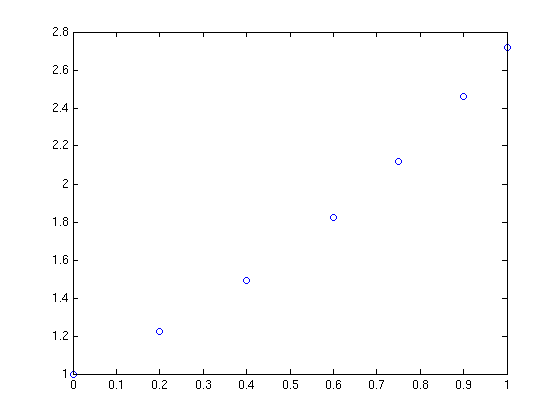
and you want to interpolate this data on a fine grid between x=0 and x=1 using piecewise cubic Hermite interpolation. One way of doing this in MATLAB is to use the interp1 function as follows

tic
t=0:0.00005:1;
y1 = interp1(x,y,t,'pchip');
toc

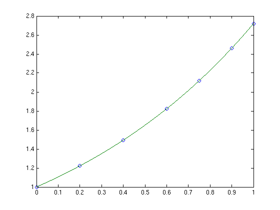
The tic and toc statements are there simply to provide timing information and on my system the above code took 0.503 seconds. We can do exactly the same calculation using the NAG toolbox for MATLAB:

tic
[d,ifail] = e01be(x,y);
[y2, ifail] = e01bf(x,y,d,t);
toc

which took 0.054958 seconds on my system making it around 9 times faster than the pure MATLAB solution – not bad at all for such a tiny amount of work.  Of course y1 and y2 are identical as the following call to norm demonstrates

norm(y1-y2)
ans =
      0

Of course the real code contained a lot more than just a call to interp1 but using the above technique decreased the run time of the user’s application from 1 hour 10 minutes down to only 26 minutes.

Thanks to the NAG technical support team for their assistance with this particular problem and to the postgraduate student who came up with the idea in the first place.

I had a query from a MATLAB user the other day and I thought I would share it with the world just in case it turned out to be useful to someone.  She had some data in a cell array that appeared as follows

data =

    '-0.000252594'
    '-0.788638'
    '-1.14636'
    '-1.15374'
    '-1.15474'

I’m not sure how she ended up with her data in this form but that’s not important here. What is important is that she couldn’t calculate with it in all the ways she was used to so what she asked was ‘how do I convert this cell array to a matrix?‘

It turns out that this is relatively easy to do since this particular cell array has a very simple form.  If you want to follow along then you can create an identical cell array as follows

data={'-0.000252594'; '-0.788638'; '-1.14636' ;'-1.15374' ;'-1.15474'}

data =

    '-0.000252594'
    '-0.788638'
    '-1.14636'
    '-1.15374'
    '-1.15474'

Let’s check that this really is a cell array using the iscell() function

iscell(data)

ans =
     1

Looks good so far. So, to convert this to a matrix all you need to do is

matdata=cellfun(@str2num,data)

matdata =
   -0.0003
   -0.7886
   -1.1464
   -1.1537
   -1.1547

the variable matdata is a standard MATLAB matrix and to prove it I’ll add 1 to all of the elements in the usual fashion

matdata+1

ans =
    0.9997
    0.2114
   -0.1464
   -0.1537
   -0.1547

That’s it! If only all queries were that simple :)

A major new release of the free alternative to MATLAB, GNU Octave was released a couple of weeks ago (on June 6th to be precise).  The Octave team have added many new features and so this release looks well worth checking out.  The full set of user visible changes can be found on the Octave website but a few highlights include.

• Compatibility with Matlab graphics has been improved – many new graphics functions added including ezplot,
  isosurface and plotmatrix.
• New functions for reading and writing images. The imwrite and imread functions have been included in Octave.
• New experimental OpenGL/FLTK based plotting system. An experimental plotting system based on OpenGL and the FLTK toolkit is now part of Octave.
• Object Oriented Programming.
• New numerical integration (quadrature) functions – dblquad, quadgk, quadv and triplequad
• Octave now includes a single precision data type. Single precision variables can be created with the single command, or from functions like ones, eye, etc.
• 64-bit integer arithmetic has been added. Arithmetic with 64-bit integers (int64 and uint64 types) is fully supported.
• Improved array indexing. The underlying code used for indexing of arrays has been completely rewritten and indexing is now significantly faster
• Various other performance improvements.
• Loads of new functions.

I recently helped someone install the new 64bit beta version of MATLAB 2009a on a dual quad core Mac pro and so far he seems very pleased with it.  The 32bit version simply didn’t cut it because he needed to be able to access huge amounts of memory.  More and more researchers at my University seem to be choosing Mac Pros over other platforms and yet it seems that the MATLAB experience on them is far from perfect (according to this link at least).

People seem to complain that its slow compared with other operating systems on comparable hardware along with a clunky user interface since it uses X11 rather than Cocoa.

I’ll lay my cards on the table – I’m not a major Mac fan – but when so many people, who’s judgement I respect, choose them over other platforms then I sit up, take notice and try to understand.  Does anyone reading this have experience with MATLAB on OS X – favourable or otherwise?

Did you know that your graphics card is effectively a mini-supercomputer?  Your main CPU (Central Processing Unit) probably has 2 processor cores, 4 if you are lucky but a high end graphics card can have as many as 96 GPUs (Graphics Processing Units) – which is a lot.  Even my laptop’s relatively low end NVIDIA GeForce 8400MS has 16 ‘stream processors‘ according to this Wikipedia page.

The large number of cheap processor cores is the good news.  The bad news is that they are not as capable as fully fledged Intel or AMD processor cores since, as you might expect, the cores in your graphics card are rather specialised.  They were designed specifically to do the mathematics behind graphics processing and they do this very well indeed but until fairly recently it was rather difficult to get them to do much else.

That hasn’t stopped people from trying though. Some time ago,NVIDIA, the makers of my laptop’s graphics card, released a software library called CUDA which enables C-programmers to access the vast computational power locked away in a typical pixel pusher.  The results have been nothing short of astonishing.  One developer, for example, recently demonstrated how to use CUDA to calculate the properties of the Ising Model (A staple in undergraduate computational physics courses) over 60 times faster than a single, bog standard Intel CPU.

If you are impressed with a factor-60 speed up then the 675 times speed up reported by Michał Januszewski and Marcin Kostur is really going to knock your socks off.  Yep – that’s not a typo.  They have written code that can solve certain Stochastic Differential Equations SIX HUNDRED AND SEVENTY FIVE TIMES FASTER than a single, standard CPU core.  Your shiny new dual quad-core workstation isn’t looking so clever now is it?  Not bad for technology designed for playing the latest version of quake on.

This is all well and good but I don’t have the time or the mental stamina to code in C anymore.  What I want is for all of my favourite Mathematica, MATLAB or Python functions to be CUDA-ised so that I can enjoy a big speed up at low cost and low programming effort.  I’ll take the moon on a stick while I’m at it if you don’t mind.

Well, it seems that some people are doing exactly this.  I have just stumbled across a project called GPUmat which claims to offer up to 40x speedup with very little effort on the part of the user.  One example they give considers the following standard MATALB code.

A = single(rand(100)); % A is on CPU memory
B = single(rand(100)); % B is on CPU memory
C = A+B;    % executed on CPU.
D = fft(C); % executed on CPU

To get this running on your graphics card all you need to do is (after you’ve installed the toolbox and CUDA of course)

A = GPUsingle(rand(100)); % A is on GPU memory
B = GPUsingle(rand(100)); % B is on GPU memory
C = A+B;    % executed on GPU.
D = fft(C); % executed on GPU

Very nice. I’m not sure what MATLAB functions are supported but I guess it’s all there in the documentation – I just haven’t had time to look through it. I’d love to tell you what sort of speed-up I experienced when I tried it out but, unfortunately, the developers are asking for all potential users to register before they get access to the downloads and that put me off a bit

It’s all free though so if you’d like to check it out yourself, and you don’t mind the registration, then head over to the developer’s website. I’d love to hear how you get on.

PS: Make sure your graphics card is CUDA compatible first though.  You’ll waste a lot of time trying out this software if it isn’t!

One of the many jobs that I have to do is to package a version of MATLAB for distribution to my employer’s standard student Windows desktop image and so I got to test MATLAB 2009a on Windows for the first time.  While testing the deployed version of MATLAB I discovered that it seemed to hang when you tried to initialise the symbolic toolbox.

For example, typing

mupad

into MATLAB should start the mupad notebook but it just sat there for over 10 minutes before I got bored and terminated the process.  Similarly, if you type

syms x

to set the variable x as a symbolic variable then it just seems to hang.  At first I thought there was something wrong with my deployment method but it turns out that it’s a bug in MATLAB 2009a.

Happily, it’s a bug that Mathworks knows about and they have provided a workaround.  Unhappily, you need to regsiter for a Mathworks account to get access to the zip file containing the workaround.

In the old days of computing, life was relatively simple as far as processor speed was concerned.  If your current computer ran at 1Ghz and you were about to buy one that ran at 2Ghz then, as a rough rule of thumb, you expected it to be about twice as fast.  Of course there was more to it than that (there always is) and other things such as amount of memory, hard disk speed etc etc also had an impact on how fast you got the results of your calculations.  It also didn’t help that not all Ghz were created equally – two chips that ran at the same clock speed but with different architectures could exhibit radically different calculation performance.

I did say life was ‘relatively simple’ not just ‘simple’.

These days we still have all of the above to worry about, but we also have the added complication that a typical modern computer contains not one, but two processors.  It’s almost like having two machines for the price of one and higher end desktops can contain as many as 8.  Which is a lot!

Back in the old, single processor, days we could take our slow code from an old machine, put it on a new machine and it would go faster.   That was it – no worries, no hassle.  If only life were so simple today….

These days we need to actually rewrite our code so that it makes better use of all the idle processors lying around in our new fangled machines or, to put it more technically, we need to parallelize our code.  Sometimes this is simple, often it’s not but one thing is for sure and that is that the environment we are programming in has to provide a set of parallel programming commands to help us do this extra work.

Old style languages such as C and FORTRAN have had this sort of stuff for years in the form of libraries such as Open MPI and Open MP but mathematical programming languages such as Mathematica and Maple have only recently gotten in on the act.

Version 7 of Mathematica and Version 13 of Maple* both included a set of tools for enabling parallel programming as part of their basic installs.  In other words – you don’t need to pay any extra money to get these programs to use your multi-processor computers to their full potential.

MATLAB, on the other hand, expects you to pay extra to be able to parallelize  your code by requiring you to purchase the Parallel Computing Toolbox.  It’s not cheap either!  Of course, Mathworks are free to charge whatever they like for their products but I don’t think that this particular policy is doing them any favours.

It’s not all bad – certain functions in basic MATLAB make full use of your multi core processors.  As of version 2009a, for example, their Fast Fourier Transform function (fft) will perform much faster on multi-processor machines but if you want to parallelize your own code then you still have to buy the Parallel toolbox.  Your alternatives include messing around with batch processing (if your problem can be solved this way) or use another package such as Mathematica or Maple which has full parallel support out of the box.

At my University we have several hundred network licenses for MATLAB itself and only 2 or 3 licenses for the Parallel toolbox.  That doesn’t mean that people aren’t interested in parallel MATLAB, quite the opposite, they simply do not want to have to pay extra to parallelize code on desktops and will go to great lengths (all legal I hasten to add) to avoid the extra cost.

Unfortunately for Mathworks one of the easiest options for someone starting on a new project is simply to use one of their competitors and this is starting to happen.  Manchester has a site license for Mathematica and I saw a big spike in interest after version 7 thanks to the parallel programming features it contains.

In summary I think that The Mathworks would do themselves a great favour by including the parallel toolbox as part of their basic package.

Any thoughts?

*Maple actually had parallel support before version 13 but it has been vastly improved in this latest version