Walking Randomly

A couple of weeks ago my friend and colleague, Ian Cottam, wrote a guest post here at Walking Randomly about his work on interfacing Dropbox with the high throughput computing software, Condor.  Ian’s post was very well received and so he’s back; this time writing about a very different kind of project.  Over to Ian.

Natural Scientists: their very big output files – and a tale of diffs by Ian Cottam

I’ve noticed that natural scientists (as opposed to computer scientists) often write, or use, programs that produce masses of output, usually just numbers. It might be the final results file or, often, some intermediate test results.

Am I being a little cynical in thinking that many users glance – ok, carefully check – a few of these thousands (millions?) of numbers and then delete the file? Let’s assume such files are really needed. A little automation is often added to the process by having a baseline file and running a program to show you the differences between it and your latest output (assuming wholesale changes are not the norm).

One of the popular difference programs is the Unix diff command . (I’ve been using it since the 1970s.) It popularised the idea of showing minimal differences between two text files (and, later, binary ones too). There are actually a few algorithms for doing minimal difference computation, and GNU diff, for example, uses a different one from the original Bell Labs version. They all have one thing in common: to achieve minimal difference computation the two files being compared must be read into main memory (aka RAM). Back in the 1970s, and on my then department’s PDP-11/40, this restricted the size of the files considerably; not that we noticed much as everything was 16bit and “small was beautiful”. GNU diff, on modern machines, can cope with very big files, but still chokes if your files, in aggregate, approach the gigabyte range.

(As a bit of an aside: a major contribution of all the GNU tools, over what we had been used to from the Unix pioneers at Bell Labs, was that they removed all arbitrary size restrictions; the most common and frustrating one being the length of text lines.)

Back to the 1970s again: Bell Labs did know that some files were too big to compare with diff , and they also shipped: diffh. The h stands for halfhearted. Diffh does not promise minimal differences, but can be very good for big files with occasional differences. It uses a pass over the files using a simple ‘sliding window’ heuristic approach (the other word that the h is sometimes said to stand for). You can still find an old version of diffh on the Internet. However, it ‘gives up’ rather easily and you may have to spend some time modifying it for, e.g., 64 bit ints and pointers, as well as for compiling with modern C compilers. Other tools exist that can compare enormous files, but they don’t produce readable output in diff’s pleasant format.

A few years back, when a user at the University of Manchester asked for help with the ‘diff – files too big/ out of memory’ problem, I wrote a modern version that I called idiffh (for Ian’s diffh). My ground rules were:

• Work on any text files on any operating system with a C compiler
• Have no limits on, e.g., line lengths or file size
• Never ‘give up’ if the going gets tough (i.e. when the files are very different)

You won’t find this with the GNU collection as they like to write code to the Unix interface and I like to write to the C standard I/O interface (see the first bullet point above).

An interesting implementation detail is that it uses random access to the files directly, relying on the operating system’s cache of file blocks to make this tolerably efficient. Waiting a minute or two to compare gigabyte sized files is usually acceptable.

As the comments in the code say, you can get some improvements by conditional compilation on Unix systems and especially on BSD Systems (including Apple Macs), but you can compile it straight, without such, on Windows and other platforms.

If you would like to try idffh out you can download it here.

A couple of years ago I wrote an article called Christmas gifts for math geeks and it has proven to be quite popular so I decided to write a follow up.  As I started thinking about what I might include, however, I started to realise that I had produced a list for science geeks instead.  So, here it is – my recommendations for gifts for the scientist in your life.

Mathematica 8 Home Edition – This is the full version of Mathematica, possibly my favourite piece of mathematical computer software, at the extremely low price of 195 pounds + VAT.  I know what you are thinking ‘Over 200 quid is not an extremely low price.’ and I would tend to agree.  It is, however, very good value since a commercial license costs several thousand pounds and Mathematica is as good as MATLAB with a whole slew of toolboxes.  Mathematica is possibly the most feature complete piece of mathematical software available today and is infinitely better than any dedicated graphical calculator.

Bigtrak – I don’t have a Bigtrak but I used to have one back in the 1980s.  Is the science geek in your life into computers and 30-40 years old?  If so then there is a distinct possibility that their first foray into the world of computer programming was with a Bigtrak back when they were 8 or so – I mean, this thing can even do loops!  This isn’t identical to the original but it is a very close facsimile and would be great for budding computer nerds or their misty eyed old dad.

200-in-1 electronic project lab.  Now this one brings back fond memories for me since it was given to me for my 10th birthday and is probably the reason I studied physics at A-Level since A-Level physics included the study of basic electronics.  I did well in A-Level physics and enjoyed it so I chose theoretical physics for my degree later moving on to a PhD so you could argue that this piece of kit changed my life!

I was overjoyed when I discovered that it was still being sold and was immensely pleased when I received it as a birthday present once again when I was 28.

The first thing you need to know about this wonderful piece of kit is that it requires no soldering; you wire up all of the components using bendy little springs – nothing could be more simple.  There is also no need to be able to read schematic diagrams (although this can be a great way to learn how to) since each spring is numbered so producing your own AM radio transmitter can be as simple as joining spring 1 to spring 10 to spring 53 and so on.

The practical upshot of all of this is that you can approach this thing at a variety of levels.  In the first instance you can just have fun building and playing with the various circuits which include things like a crystal set radio, a Morse code transmitter, a light detector, a sound detector and basic electronic games.  Once you’ve got that out of your system you can start to learn the basics of electronics if you wish.

I have since discovered 300 in 1 and even 500 in 1 electronic project labs which look great and all but this is the one that will forever be in my heart.

Wonders of the Solar System – I have always loved (although never practised) astronomy and avidly followed the adventures of Voyagers 1 and 2 when I was small.  Since then, modern space probes such as Cassini-Huygens, Galileo and Mars Odyssey have added more to our knowledge of our astronomical backyard  and we now know a tremendous amount about the solar system.  In this series, Brian Cox of the University of Manchester takes us on a grand-tour around the solar system.  The imagery is fantastic, Cox’s enthusiasm is infectious and the science is awesome.  Yep, I quite like this DVD :)

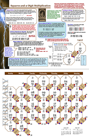
2011 ‘Lightning Calculation’ calendar – Ron Doerfler writes a blog called Dead Reckonings that specialises in the lost arts of the mathematical sciences.  Last year he designed a 2010 Graphical Computing calendar and made the designs available for free to allow you to print your own.  Centred around ancient computing devices called nomograms, the calendar was beautiful and after Ron very kindly sent me a copy, I encouraged him to make a version that he could sell.  Well, I guess he took my advice because Ron is back with a 2011 calendar with the theme of ‘Lightning Calculations’ and this time he is selling it from Lulu.com.

Since Ron is an all round nice guy, he also offers a high resolution pdf of the calendar to allow you to print it off yourself but personally I plan on showing my support by putting an order in with Lulu.com.  Nice work Ron!

I work for a large university in the UK and part of my job involves helping to look after our site licenses for software such as MATLAB, Origin, Labview, Mathematica,Abaqus and the NAG Library among many others.  Now, anyone who works in this field will know that no two site licenses are alike.  For example, one license might allow any member of the university to install it on any machine that they own whereas others are limited only to university owned machines.  There are lots of little rules like this and I could go on for quite a while about some of the gotchas but I’d prefer to focus this post on something close to my heart right now – the matter of perpetual usage.

Imagine, if you will, that you are the coordinator for a degree course and you are completely overhauling the  syllabus.  Part of this overhaul will concern the software that you use and teach as part of this course.  You want to standardize on just one package so that students won’t have to learn a new system every semester.  After reviewing all of the possibilities, you finally decide that it is going to be either software A or software B.  Both are powerful, easy to use, considered an industry standard etc etc.  As far as functionality goes there really isn’t much between them.  Which one to choose?

You invite your friendly,neighborhood software geek out for coffee and ask him to talk about the two software packages.  He likes talking about this sort of stuff and usually has a lot to say.  He talks about open-source alternatives, programming styles, speed, potentially useful books, other people in your field who use this type of software and so on.  Eventually he starts talking about licensing and offers the following tidbit of information.

• Our license for Software A includes perpetual use.  This means that if our funding dried up we could stop paying our maintenance agreement but we would never lose access to the software.  Of course we’d not be able to upgrade to the latest version any more but we’d always have access to the version we have right now.
• Our license for Software B doesn’t include perpetual use.  So, if we stopped paying our maintenance agreement then we can’t use the software anymore.  We’d have to stop using it for teaching, research….everything.  You’d have to go and buy your own license for it.

“How likely is it that we might stop funding either of them?” you ask.

“Oh, pretty unlikely,” comes the reply as he rests his coffee mug over that day’s newspaper headline “We are a big university and both of these packages are key to what we do.  I’d say we are very unlikely to stop funding either of them.”

I have a question to you all.  Would the lack of perpetual use for Software B be a factor in your decision concerning what you would use for your teaching and research?

This is not a serious post but then mathematics doesn’t have to be serious all the time does it?  Ever wondered what the equation of a 3D heart looks like?  An old post of mine will help you find the answer using Mathematica.  Click on the image for more details (and a demonstration that you can run using the free Mathematica player).

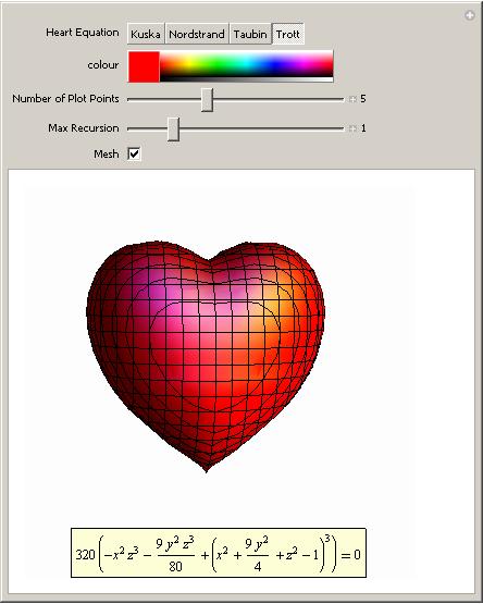
I don’t save all of my love for Mathematica though. I’ve got some for MATLAB too:

%code to plot a heart shape in MATLAB
%set up mesh
n=100;
x=linspace(-3,3,n);
y=linspace(-3,3,n);
z=linspace(-3,3,n);
[X,Y,Z]=ndgrid(x,y,z);
%Compute function at every point in mesh
F=320 * ((-X.^2 .* Z.^3 -9.*Y.^2.*Z.^3/80) + (X.^2 + 9.* Y.^2/4 + Z.^2-1).^3);
%generate plot
isosurface(F,0)
view([-67.5 2]);

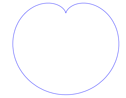
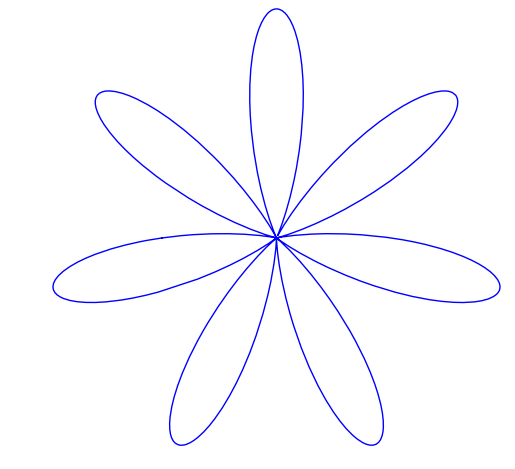
Did you know that the equation for a heart (or a cardioid if you want to get technical) is very similar to the equation for a flower?  The polar equation you need is  and you get a rotated cardioid for n=1.  Change n to 6 and you get a flower.  Let’s use the free maths package, SAGE, this time.

First, define the function:

def eqn(x,n):
    return(1-sin(n*x))

then plot it for n=1

polar_plot(eqn(x,1), (x,-pi, pi),aspect_ratio=1,axes=False)

and for n=7

polar_plot(eqn(x,7), (x,-pi, pi),aspect_ratio=1,axes=False)

Back to Mathematica and the Wolfram Demonstrations project. We have a Valentine’s version of the traditional Tangram puzzle.

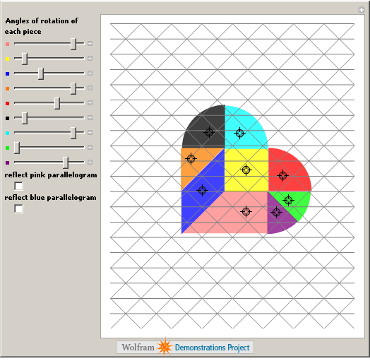
Feel free to let me know of any other Valentine’s math that you discover, puzzles, fractals or equations, it’s all good :)

Update Feb 14th 2011

Mariano Beguerisse Díaz sent me some MATLAB code that uses a variation on the standard mandelbrot and I turned it into the movie below.  His original code is in the comments section

This is the first post on Walking Randomly that isn’t written by me!  I’ve been thinking about having guest writers on here for quite some time and when I first saw the tutorial below (written by Manchester University undergraduate, Gregory Astley) I knew that the time had finally come.  Greg is a student in Professor Bill Lionheart’s course entitled Asymptotic Expansions and Perturbation Methods where Mathematica is the software of choice.

Now, students at Manchester can use Mathematica on thousands of machines all over campus but we do not offer it for use on their personal machines.  So, when Greg decided to write up his lecture notes in Latex he needed to come up with an alternative way of producing all of the plots and he used the free, open source computer algebra system – Maxima.  I was very impressed with the quality of the plots that he produced and so I asked him if he would mind writing up a tutorial and he did so in fine style.  So, over to Greg….

This is a short tutorial on how to get up and running with the “plotdf” function for plotting direction fields/trajectories for 1st order autonomous ODEs in Maxima. My immediate disclaimer is that I am by no means an expert user!!! Furthermore, I apologise to those who have some experience with this program but I think the best way to proceed is to assume no prior knowledge of using this program or computer algebra systems in general.  Experienced users (surely more so than me) may feel free to skip the ‘boring’ parts.

Firstly, to those who may not know, this is a *free* (in both the “costs no money”, and “it’s open source” senses of the word) computer algebra system that is available to download on Windows, Mac OS, and Linux platforms from  http://maxima.sourceforge.net and it is well documented.

There are a number of different themes or GUIs that you can use with the program but I’ll assume we’re working with the somewhat basic “Xmaxima” shell.

Install and open up the program as you would do with any other and you will be greeted by the following screen.

You are meant to type in the top most window next to (%i1) (input 1)
We first have to load the plotdf package (it isn’t loaded by default) so type:

load("plotdf");

and then press return (don’t forget the semi-colon or else nothing will happen (apart from a new line!)). it should respond with something similar to:

(%i1)  load("plotdf");
(%o1)  /usr/share/maxima/5.17.1/share/dynamics/plotdf.lisp
(%i2)

We will now race ahead and do our first plot. Keeping things simple for now we’ll do a phase plane plot for dx/dt = y, dy/dt = x, type:

plotdf([y,x]);

you should see something like this:

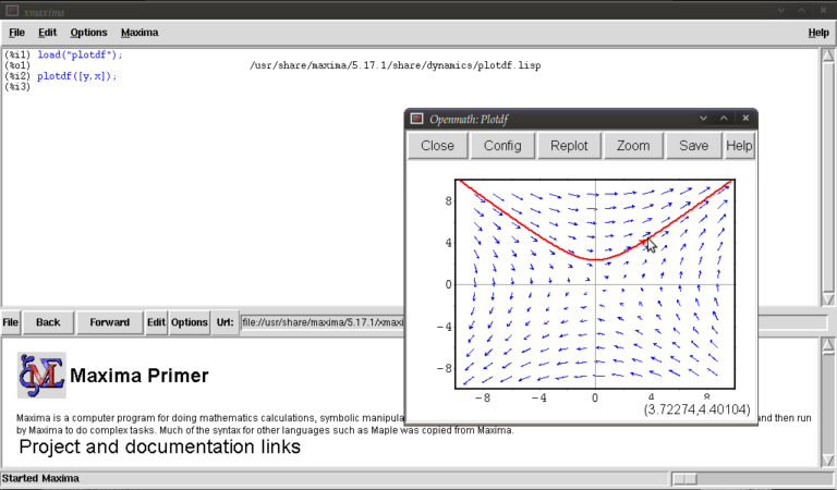
This is the Openmath plot window, (there are other plotting environments like Gnuplot but this function works only with Openmath) Notice that my pointer is directly below a red trajectory. These plots are interactive, you can draw other trajectories by clicking elsewhere. Try this.  Hit the “replot” button and it will redraw the direction field with just your last trajectory.

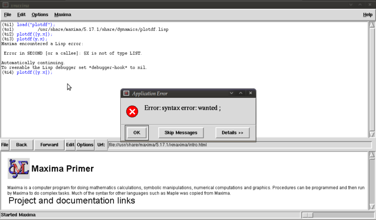
Before exploring any other options I want to purposely type some bad input and show how to fix things when it throws an error or gets stuck. Type

plotdf(y,x);

it should return

(%i3) plotdf(x,y);
Maxima encountered a Lisp error:

Error in SECOND [or a callee]: $Y is not of type LIST.

Automatically continuing.
To enable the Lisp debugger set *debugger-hook* to nil.
(%i4)

We forgot to put our functions for dx/dt,dy/dt in a list (square brackets). This is a reasonably safe error in that it tells us it isn’t happy and lets us continue.
Now type

plotdf([x.y]);

you should see something similar to

The problem this time was that we typed a dot instead of a comma (easily done), but worryingly when we close this message box and the blank plot the program will not process any commands. This can be fixed by clicking on the following in the xmaxima menu

file >> interrupt

where after telling you it encountered an error it should allow you to continue. One more; type

plotdf([2y,x]);

It should return with

  (%i5) plotdf([2y,x]);
  Incorrect syntax: Y is not an infix operator
  plotdf([2y,
           ^
  (%i5)

This time we forgot to put a binary operation such as * or + between 2 and y. If you come up with any other errors and the interrupt command is of no use you can still partially salvage things via

  file >> restart

but you will, in this case, have to load plotdf again. (mercifully you can go to the line where you first typed it and press return (as with other commands you might have done))
I will now demonstrate some more “contrived” plots (for absolutely no purpose other than to shamelessly give a (very) small gallery of standard functions/operations etc… for the novice user) there is no need to type the last four unless you want to see what happens by changing constants/parameters, they’re the same plot :)

  plotdf([2*y-%e^(3/2)+cos((%pi/2)*x),log(abs(x))-%i^2*y]);
  plotdf([integrate(2*y,y)/y,diff((1/2)*x^2,x)]);
  plotdf([(3/%pi)*acos(1/2)*y,(2/sqrt(%pi))*x*integrate(exp(-x^2),x,0,inf)]);
  plotdf([floor(1.43)*y,ceiling(.35)*x]);
  plotdf([imagpart(x+%i*y),(sum(x^n,n,0,2)-sum(x^j,j,0,1))/x]);

I could go on…notice that the constants pi, e, and i are preceded by “%”. This tells maxima that they are known constants as opposed to symbols you happened to call “pi”, “e”, and “i”. Also, noting that the default range for x and y is (-10,10) in both cases; feel free to replot the first of those five without wrapping x inside “abs()” (inside the logarithm that is). remember file >> interrupt afterwards!

Now I will introduce you to some more of the parameters you can plug into “plotdf(…)”. close any plot windows and type

plotdf([x,y],[x,1,5],[y,-5,5]);

You should notice that x now ranges from 1 to 5, whilst y ranges from -5 to 5. There is nothing special about these numbers, we could have chosen any *real* numbers we liked. You can also use different symbols for your variables instead of x or y. Try

plotdf([v,u],[u,v]);

Note that I’ve declared u and v as variables in the second list. I will now purposely do something wrong again. Assign the value 5 to x by typing

x:5;

then type

plotdf([y,x]);

This time maxima won’t throw an error because syntactically you haven’t done anything wrong, you merely told it to do

plotdf([y,5]);

as opposed to what you really wanted which is

plotdf([y,x]);

Surprisingly to me (discovered as I’m writing this), changing the names of your variables like we did above won’t save you since it seems to treat new symbols as merely placeholders for it’s favourite symbols x and y. To get round this type

kill(x);

and this will put x back to what it originally was (the symbol x as opposed to 5).
You don’t actually have to provide expressions for dx/dt and dy/dt, you might instead know dy/dx and you can generate phaseplots by typing say

plotdf([x/y]);

In this case we didn’t actually need the square brackets because we are providing only one parameter: dy/dx (x will be set to t by maxima giving dx/dt = 1, and dy/dt = dy/dx = x/y)

A number of parameters can be changed from within the openmath window. Type

plotdf([y,x],[trajectory_at,-1,-2],[direction,forward]);

and then go into config. The screen you get should look something like this:

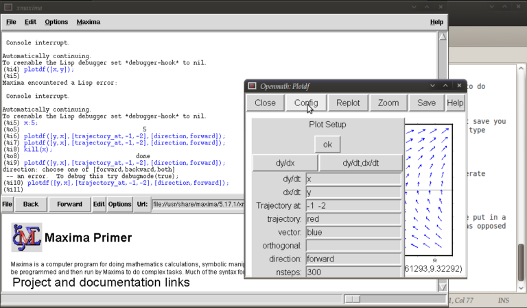
from here you can change the expressions for dx/dt, dy/dt, dy/dx, you can change colours and directions of trajectories (choices of forward, backward, both), change colours for direction arrows and orthogonal curves, starting points for trajectories (the two numbers separated by a space here, not a comma), time increments for t, number of steps used to create an integral curve. You can also look at an integral plots for x(t) and y(t) corresponding to the starting point given (or clicked) by hitting the “plot vs t” button. You can also zoom in or out by hitting the “zoom” button and clicking (or shift+clicking to unzoom), doing something else like hitting the config button will allow you to quit being in zoom mode click for trajectories again. (there might be a better way of doing this btw) You can also save these plots as eps files (you can then tweak these in other vector graphics based programs like Inkscape (free) or Adobe Illustrator etc..)

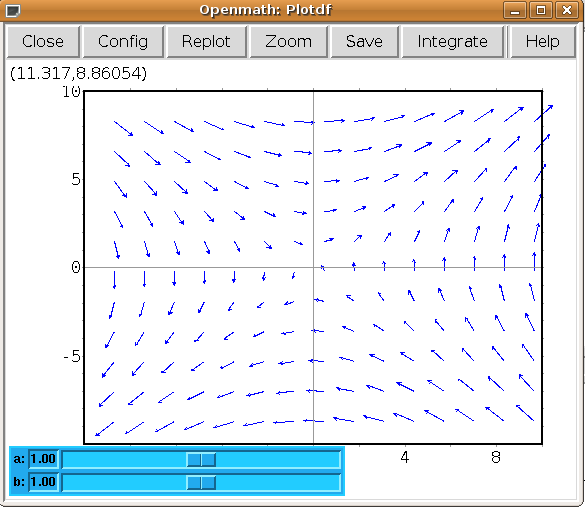
Interactive sliders

There are many permutations of things you can do (and you will surely find some of these by having a play) but my particular favourite is the option to use sliders allowing you to vary a parameter interactively and seeing what happens to the trajectories without constant replotting. ie:

plotdf([a*y,b*x],[sliders,"a=-1:3,b=-1:3"]);

Hopefully, this has been enough to get people started, and for what it’s worth, the help file (though using xmaxima, you’ll find this in the web-browser version) for this topic has a pretty good gallery of different plots and other parameters I didn’t mention.

just to throw in one last thing in the spirit of experimentation, is the following set of commands:

A:matrix([0,1],[1,0]);
B:matrix([x],[y]);
plotdf([A[1].B,A[2].B);

which is another way of doing the same old

plotdf([y,x]);

where here I’ve made a 2×2 matrix A, a 2×1 matrix B, with A[1], A[2] denoting rows 1 and 2 of A respectively and matrix multiplied the rows of A by B (using A[1].B, A[2].B) to serve as inputs for dx/dt and dy/dt

Tutorial written by Gregory Astley, Mathematics Undergraduate at The University of Manchester.

Within every field of human endeavor there is a collection of Holy Grail-like accomplishments; achievements so great that the attainment of any one of them would instantly guarantee a place in the history books. In Physics, for example, there is the discovery of the Higgs boson or room temperature superconductivity; Medicine has the cure for cancer and how to control the ageing process whereas Astronomy has dark matter and the discovery of extra-solar planets that are capable of supporting life.

Of course, mathematics is no exception and its Holy Grail set of exploits include problems such as the proof of the Riemann hypothesis, the Goldbach conjecture and the Collatz Problem.  In the year 2000, The Clay Mathematics Institute chose seven of what it considered to be the most important unsolved problems in mathematics and offered $1 million for the solution of any one of them.  These problems have since been referred to as The Millenium Prize Problems and many mathematicians thought that it would take several decades before even one was solved.

Just three years later, Grigori Perelman solved the first of them –  The Poincaré conjecture.  Stated over 100 years ago (in 1904 to be exact) by Henri Poincaré, the conjecture says that ‘Every simply connected closed three-manifold is homeomorphic to the three-sphere’.  If, like me, you struggle to understand what that actually means then an alternative statement provided by Wolfram Alpha might help – ‘The three-sphere is the only type of bounded three-dimensional space possible that contains no holes.’  99 years later, after generations of mathematicians tried and failed to prove this statement, Perelman published a proof on the Internet that has since been verified as correct by several teams of mathematicians.  For this work he was awarded the Field’s Medal, one of the highest awards in mathematics, which he refused.  According to Wolfram Alpha, Perelman also refused the $1 million from the Clay Institute but, as far as I know at least, he has not yet been offered it (can anyone shed light on this matter?).

Yep, Girgori Perelman is clearly rather different from most of us.  Not only is he obviously one of the most gifted mathematicians in the world but he also sees awards such as the Field’s Medal very differently from many of us (after all, would YOU refuse such an award – I know I wouldn’t!).  So, what kind of a man is he?  How did he become so good at mathematics and why did he turn down such prestigious prizes?

In her book, Perfect Rigor, Masha Gessen attempts to answer these questions and more besides by writing a biography of Perelman.  Starting before he was even born, Gessen tells Perelman’s story in the words of those who know him best – his friends, colleagues and competitors.  Unfortunately, we never get to hear from the man himself because he cut off all communications with journalists before Gessen started researching the book.  Despite this handicap, I think that she has done an admirable job and by the end of it I have a feeling that I understand Perelman and his motives a little better than before.

This is not a book about mathematics, it is a book about people who DO mathematics and gives an insight into the pressures, joys and politics that surround the subject along with what it was like to be a Jewish mathematician in Soviet-era Russia.  What’s more, it is absolutely fascinating and I devoured it in just a few commutes to and from work.  With hardly an equation in sight, you don’t need pencil and paper to follow the story (unlike many of the books I read on mathematics), all you need is a few hours and somewhere to relax.

The only problem I have with this book is that by the end of it I didn’t feel like I knew much more about the Poincaré conjecture itself despite getting to know its conqueror a whole lot more.  Since I didn’t know much (Oh Ok…anything) about it to start with this is a bit of a shame.  Near the end of writing this review, I took a look at what reviewers on Amazon.com thought of it and it seems that some of them are also disappointed at the mathematical content of the book and they come from a position of some authority on the subject.  The best I can say is that if you want to learn about the Poincaré conjecture then this probably isn’t the book for you.

If, on the other hand, you want to learn more about the human being who slayed one of the most difficult mathematical problems of the millennium then I recommend this book wholeheartedly.

It never ceases to amaze me how researchers manage to find connections between the most seemingly disconnected of things.  A researcher at Manchester University, Bill Lionheart, conducts research into the mathematics of ‘seeing inside things with electricty’ and over at his blog he has a great story which basically says that a certain breed of fish are significantly better at this particular branch of mathematics than we are.

One particular quote I love is “Weakly electric fish are really interesting to us because they have the ability to solve a challenging mathematical problem when catching their food.” as it made me wonder how students would feel if they had to solve challenging mathematical problems in order to get their food :)

An algebraic surface is a set of solutions to the general equation f(x,y,z)=0 where f is a polynomial in the variables x,y and z.  For example if you set f to the following polynomial

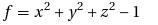
then the set of points x,y and z that satisfy f(x,y,z)=0 forms a sphere of radius 1.  You can get much more interesting surfaces than a sphere though.  For example, set

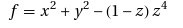
and you’ll get something known as the kiss surface – so called because the bottom section resembles a Hershey’s Kiss. Wolfram Alpha knows all about this surface and if you wolf Kiss Surface you’ll get a whole load of mathematical information about it along with the plot below.

One algebraic surface I have looked at in the past is the Heart Surface and it’s pretty obvious to see where it gets its name from.

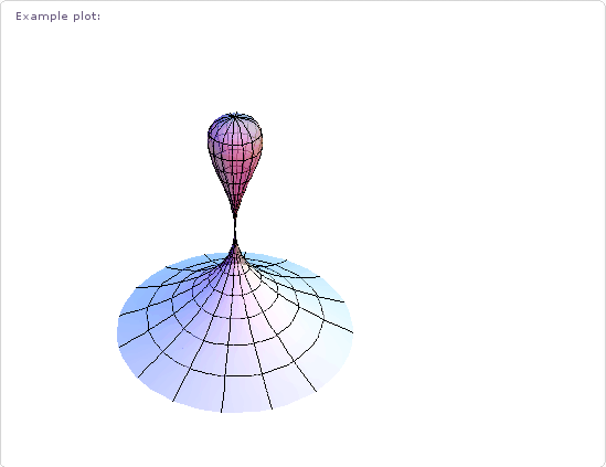
At the time of writing, Wolfram Alpha knows about 129 different, named algebraic surfaces but for some of them it can be a little harder to work out how they got their name. Does anyone know why the one below is called the Flirt Surface for example?

Other interesting ones have names like Heaven and Hell,Citrus, Star and Plop!

This functionality is very nice indeed but for it to be really impressive I’d like to see a bit more (I wouldn’t be me if I didn’t want more). For example, it would be great if I could rotate each surface with the mouse – just as I can with 3D images in Mathematica. I’d also like to see more information on each surface such as how it got it’s name or the Mathematica code needed to produce the plot.

What’s your favourite algebraic surface and what extra functionality would you like to see in this area?

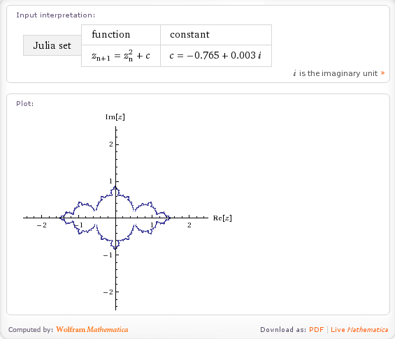
I saw a tweet from someone this morning which mentioned that you could plot the Julia Set using Wolfram Alpha.  I had to try this for myself as soon as I could and, sure enough, you can plot the Julia set for any complex number Z: -0.765+0.003 I for example.

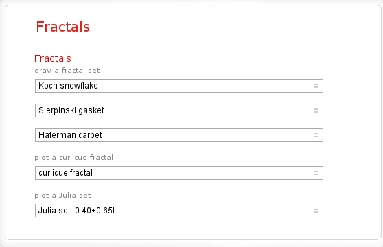
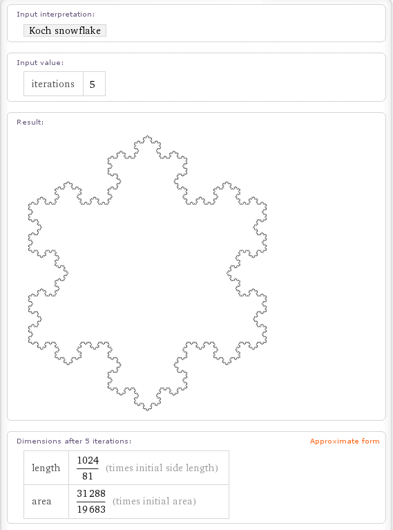
Very nice but what else can it do.  If I Walpha fractals then I get the following output so I’d expect Wolfram Alpha to compute at least the Koch snow flake, the Sierpinski gasket, the Haferman carpet and the curlicue fractal and, sure enough, it does (click on the links to see for yourself)

Here is a screenshot for the Koch Fractal.

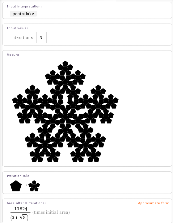
These aren’t the only fractals it knows about though. If you walpha Pentaflake (a fractal close to my heart) then you get the following.

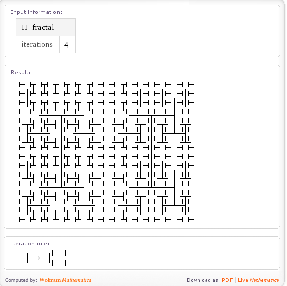
Wolfram Alpha can also calculate the H-Fractal.

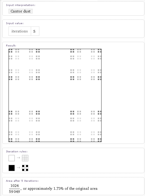
Cantor dust is in there too

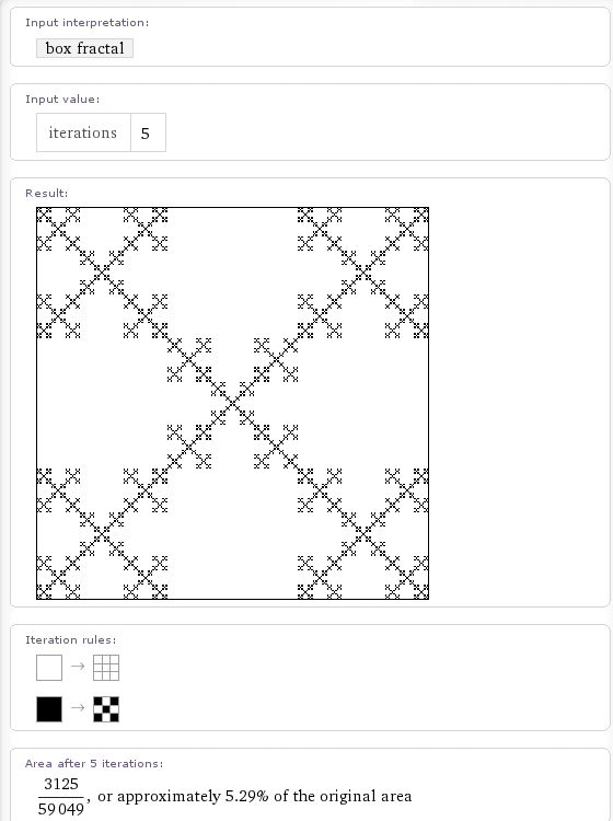
as is the box fractal

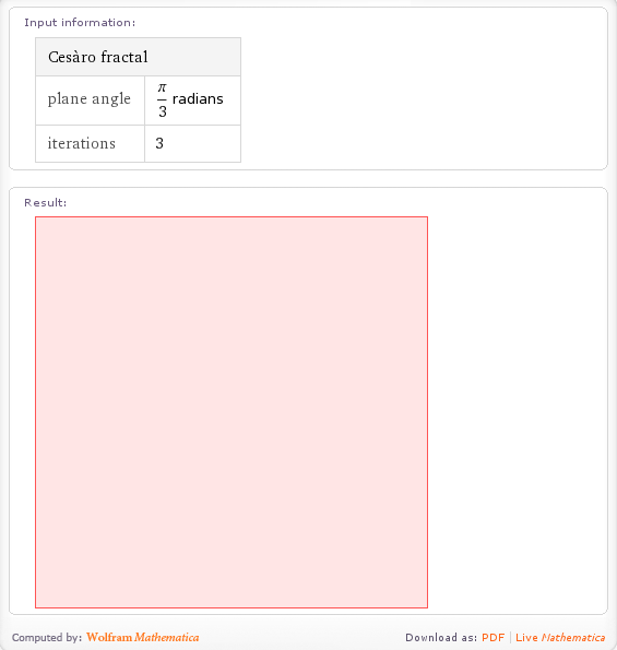
It also looks like they are in the middle of implementing the Cesaro fractal.  If you walpha the term then it tries to generate the fractal for a phase angle of pi/3 radians and 5 iterations.  A few seconds later and the calculation times out.  If you lower the number of iterations it returns a red box such as the one below.  If my memory serves, Mathematica returns such a box if there is a problem with the graphics output.  I hope to see this fixed soon.

Update:15th July 2009 – The Cesaro Fractal has now been fixed)

It also seems to know about the following fractals but doesn’t seem to calculate anything for them (yet).  I say that it seems to know about them because it gives you an input field for ‘Iterations’ which implies that it knows that a number of iterations makes sense in this context.  It’ll be cool to see all of these implemented in time.

(Note: None of these are implemented yet and may never be – I’ll update if that changes)

• Menger Sponge Update 21st December 2010 – this has now been implemented
• Gosper Island Update:15th July 2009 – this has now been implemented
• Apollonian Gasket Update 21st December 2010 – this has now been implemented
• Dragon Curve Update 21st December 2010 – this has now been implemented
• Hilbert Curve Update 21st December 2010 – this has now been implemented
• Peano curve Update 21st December 2010 – this has now been implemented
• Cantor Set Update:15th July 2009 – this has now been implemented

Some odd omissions (at the time of writing) are the Mandelbrot set (Update: 15th July 2009 – this has been done now) and the Lorenz attractor.

This is all seriously cool stuff for Fractal fans and shows the power of the Wolfram Alpha idea.  Let me know if you discover any more Fractals that it knows about and I’ll add them here.

Update: I’ve found a few more computable fractals in Wolfram Alpha.  Please forgive me for the lack of screenshots but this is getting to be a rather graphic-intensive post.  The links will take you to a Wolfram Alpha query.

• Levy Fractal
• Levy Tapestry
• Pythagoras tree
• Koch Antisnowflake

Back in February I blogged about a little Mathematica demonstration I wrote which plotted several heart shaped algebraic surfaces. One or two people wrote in the comments section asking how to do such plots in MATLAB and I thought that it was about time I came up with the code.

%code to plot a heart shape in MATLAB
%set up mesh
n=100;
x=linspace(-3,3,n);
y=linspace(-3,3,n);
z=linspace(-3,3,n);
[X,Y,Z]=ndgrid(x,y,z);
%Compute function at every point in mesh
F=320 * ((-X.^2 .* Z.^3 -9.*Y.^2.*Z.^3/80) + (X.^2 + 9.* Y.^2/4 + Z.^2-1).^3);
%generate plot
isosurface(F,0)
view([-67.5 2]);


It’s not really the right time of year for hearts though is it? So let’s plot a star instead.


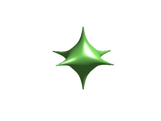
%Code to plot a 3D star in MATLAB
%set up mesh
n=200;
x=linspace(-2,2,n);
y=linspace(-2,2,n);
z=linspace(-2,2,n);
[X,Y,Z]=ndgrid(x,y,z);
%Compute function at every point in mesh
F=X.^2+Y.^2+Z.^2+1000*(X.^2+Y.^2).*(X.^2+Z.^2).*(Y.^2+Z.^2);
%generate plot
isosurface(F,1);
axis off;
view([-48 18]);


For more examples of algebraic surfaces see the Algebraic Surfaces Gallery.