Walking Randomly

My stepchildren are pretty good at mathematics for their age and have recently learned about Pythagora’s theorem

$c=\sqrt{a^2+b^2}$

The fact that they have learned about this so early in their mathematical lives is testament to its importance. Pythagoras is everywhere in computational science and it may well be the case that you’ll need to compute the hypotenuse to a triangle some day.

Fortunately for you, this important computation is implemented in every computational environment I can think of!
It’s almost always called hypot so it will be easy to find.
Here it is in action using Python’s numpy module

import numpy as np
a = 3
b = 4
np.hypot(3,4)

5

When I’m out and about giving talks and tutorials about Research Software Engineering, High Performance Computing and so on, I often get the chance to mention the hypot function and it turns out that fewer people know about this routine than you might expect.

Trivial Calculation? Do it Yourself!

Such a trivial calculation, so easy to code up yourself! Here’s a one-line implementation

def mike_hypot(a,b):
    return(np.sqrt(a*a+b*b))

In use it looks fine

mike_hypot(3,4)

5.0

Overflow and Underflow

I could probably work for quite some time before I found that my implementation was flawed in several places. Here’s one

mike_hypot(1e154,1e154)

inf

You would, of course, expect the result to be large but not infinity. Numpy doesn’t have this problem

np.hypot(1e154,1e154)

1.414213562373095e+154

My function also doesn’t do well when things are small.

a = mike_hypot(1e-200,1e-200)

0.0

but again, the more carefully implemented hypot function in numpy does fine.

np.hypot(1e-200,1e-200)

1.414213562373095e-200

Standards Compliance

Next up — standards compliance. It turns out that there is a an official standard for how hypot implementations should behave in certain edge cases. The IEEE-754 standard for floating point arithmetic has something to say about how any implementation of hypot handles NaNs (Not a Number) and inf (Infinity).

It states that any implementation of hypot should behave as follows (Here’s a human readable summary https://www.agner.org/optimize/nan_propagation.pdf)

hypot(nan,inf) = hypot(inf,nan) = inf

numpy behaves well!

np.hypot(np.nan,np.inf)

inf

np.hypot(np.inf,np.nan)

inf

My implementation does not

mike_hypot(np.inf,np.nan)

nan

So in summary, my implementation is

• Wrong for very large numbers
• Wrong for very small numbers
• Not standards compliant

That’s a lot of mistakes for one line of code! Of course, we can do better with a small number of extra lines of code as John D Cook demonstrates in the blog post What’s so hard about finding a hypotenuse?

Hypot implementations in production

Production versions of the hypot function, however, are much more complex than you might imagine. The source code for the implementation used in openlibm (used by Julia for example) was 132 lines long last time I checked. Here’s a screenshot of part of the implementation I saw for prosterity. At the time of writing the code is at https://github.com/JuliaMath/openlibm/blob/master/src/e_hypot.c

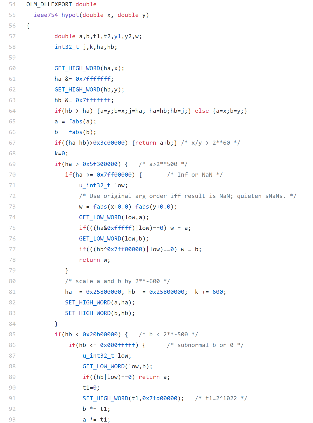
That’s what bullet-proof, bug checked, has been compiled on every platform you can imagine and survived code looks like.

There’s more!

Active Research

When I learned how complex production versions of hypot could be, I shouted out about it on twitter and learned that the story of hypot was far from over!

The implementation of the hypot function is still a matter of active research! See the paper here https://arxiv.org/abs/1904.09481

Is Your Research Software Correct?

Given that such a ‘simple’ computation is so complicated to implement well, consider your own code and ask Is Your Research Software Correct?.

In many introductions to numpy, one gets taught about np.ones, np.zeros and np.empty. The accepted wisdom is that np.empty will be faster than np.ones because it doesn’t have to waste time doing all that initialisation. A quick test in a Jupyter notebook shows that this seems to be true!

import numpy as np

N = 200
zero_time = %timeit -o some_zeros = np.zeros((N,N))
empty_time = %timeit -o empty_matrix = np.empty((N,N))
print('np.empty is {0} times faster than np.zeros'.format(zero_time.average/empty_time.average))


8.34 µs ± 202 ns per loop (mean ± std. dev. of 7 runs, 100000 loops each)
436 ns ± 10.6 ns per loop (mean ± std. dev. of 7 runs, 1000000 loops each)
np.empty is 19.140587654682545 times faster than np.zeros

20 times faster may well be useful in production when using really big matrices. Might even be worth the risk of dealing with uninitialised variables even though they are scary!

However…..on my machine (Windows 10, Microsoft Surface Book 2 with 16Gb RAM), we see the following behaviour with a larger matrix size (1000 x 1000).

import numpy as np

N = 1000
zero_time = %timeit -o some_zeros = np.zeros((N,N))
empty_time = %timeit -o empty_matrix = np.empty((N,N))
print('np.empty is {0} times faster than np.zeros'.format(zero_time.average/empty_time.average))


113 µs ± 2.97 µs per loop (mean ± std. dev. of 7 runs, 10000 loops each)
112 µs ± 1.01 µs per loop (mean ± std. dev. of 7 runs, 10000 loops each)
np.empty is 1.0094651980894993 times faster than np.zeros

The speed-up has vanished! A subsequent discussion on twitter suggests that this is probably because the operating system is zeroing all of the memory for security reasons when using numpy.empty on large arrays.

What is Second Order Cone Programming (SOCP)?

Second Order Cone Programming (SOCP) problems are a type of optimisation problem that have applications in many areas of science, finance and engineering. A summary of the type of problems that can make use of SOCP, including things as diverse as designing antenna arrays, finite impulse response (FIR) filters and structural equilibrium problems can be found in the paper ‘Applications of Second Order Cone Programming’ by Lobo et al. There are also a couple of examples of using SOCP for portfolio optimisation in the GitHub repository of the Numerical Algorithms Group (NAG).

A large scale SOCP solver was one of the highlights of the Mark 27 release of the NAG library (See here for a poster about its performance). Those who have used the NAG library for years will expect this solver to have interfaces in Fortran and C and, of course, they are there. In addition to this is the fact that Mark 27 of the NAG Library for Python was released at the same time as the Fortran and C interfaces which reflects the importance of Python in today’s numerical computing landscape.

Here’s a quick demo of how the new SOCP solver works in Python. The code is based on a notebook in NAG’s PythonExamples GitHub repository.

NAG’s handle_solve_socp_ipm function (also known as e04pt) is a solver from the NAG optimization modelling suite for large-scale second-order cone programming (SOCP) problems based on an interior point method (IPM).

$$
\begin{array}{ll}
{\underset{x \in \mathbb{R}^{n}}{minimize}\ } & {c^{T}x} \\
\text{subject to} & {l_{A} \leq Ax \leq u_{A}\text{,}} \\
& {l_{x} \leq x \leq u_{x}\text{,}} \\
& {x \in \mathcal{K}\text{,}} \\
\end{array}
$$

where $\mathcal{K} = \mathcal{K}^{n_{1}} \times \cdots \times \mathcal{K}^{n_{r}} \times \mathbb{R}^{n_{l}}$ is a Cartesian product of quadratic (second-order type) cones and $n_{l}$-dimensional real space, and $n = \sum_{i = 1}^{r}n_{i} + n_{l}$ is the number of decision variables. Here $c$, $x$, $l_x$ and $u_x$ are $n$-dimensional vectors.

$A$ is an $m$ by $n$ sparse matrix, and $l_A$ and $u_A$ and are $m$-dimensional vectors. Note that $x \in \mathcal{K}$ partitions subsets of variables into quadratic cones and each $\mathcal{K}^{n_{i}}$ can be either a quadratic cone or a rotated quadratic cone. These are defined as follows:

• Quadratic cone:

$$
\mathcal{K}_{q}^{n_{i}} := \left\{ {z = \left\{ {z_{1},z_{2},\ldots,z_{n_{i}}} \right\} \in {\mathbb{R}}^{n_{i}} \quad\quad : \quad\quad z_{1}^{2} \geq \sum\limits_{j = 2}^{n_{i}}z_{j}^{2},\quad\quad\quad z_{1} \geq 0} \right\}\text{.}
$$

• Rotated quadratic cone:

$$
\mathcal{K}_{r}^{n_{i}} := \left\{ {z = \left\{ {z_{1},z_{2},\ldots,z_{n_{i}}} \right\} \in {\mathbb{R}}^{n_{i}}\quad\quad:\quad \quad\quad 2z_{1}z_{2} \geq \sum\limits_{j = 3}^{n_{i}}z_{j}^{2}, \quad\quad z_{1} \geq 0, \quad\quad z_{2} \geq 0} \right\}\text{.}
$$

For a full explanation of this routine, refer to e04ptc in the NAG Library Manual

Using the NAG SOCP Solver from Python

This example, derived from the documentation for the handle_set_group function solves the following SOCP problem

minimize $${10.0x_{1} + 20.0x_{2} + x_{3}}$$

from naginterfaces.base import utils
from naginterfaces.library import opt

# The problem size:
n = 3

# Create the problem handle:
handle = opt.handle_init(nvar=n)

# Set objective function
opt.handle_set_linobj(handle, cvec=[10.0, 20.0, 1.0])

# Set box constraints
opt.handle_set_simplebounds(
    handle,
    bl=[-2.0, -2.0, -1.e20],
    bu=[2.0, 2.0, 1.e20]
)

# Set linear constraints
opt.handle_set_linconstr(
    handle,
    bl=[-1.e20, 1.0],
    bu=[1.5, 1.e20],
    irowb=[1, 1, 1, 2, 2, 2],
    icolb=[1, 2, 3, 1, 2, 3],
    b=[-0.1, -0.1, 1.0, -0.06, 1.0, 1.0]
    );

# Set cone constraint
opt.handle_set_group(
    handle,
    gtype='Q',
    group=[ 3,1, 2],
    idgroup=0
);

# Set some algorithmic options.
for option in [
        'Print Options = NO',
        'Print Level = 1'
]:
    opt.handle_opt_set(handle, option)

# Use an explicit I/O manager for abbreviated iteration output:
iom = utils.FileObjManager(locus_in_output=False)

# Call SOCP interior point solver
result = opt.handle_solve_socp_ipm(handle, io_manager=iom)

 ------------------------------------------------
  E04PT, Interior point method for SOCP problems
 ------------------------------------------------

 Status: converged, an optimal solution found
 Final primal objective value -1.951817E+01
 Final dual objective value   -1.951817E+01

result.x

array([-1.26819151, -0.4084294 ,  1.3323379 ])

and the objective function value is

result.rinfo[0]

-19.51816515094211

Finally, we clean up after ourselves by destroying the handle

# Destroy the handle:
opt.handle_free(handle)

As you can see, the way to use the NAG Library for Python interface follows the mathematics quite closely.
NAG also recently added support for the popular cvxpy modelling language that I’ll discuss another time.

Links

• SOCP examples on NAG’s GitHub page
• Poster discussing performance of the NAG SOCP solver

I am a huge user of Anaconda Python and the way I usually get access to the Anaconda Prompt is to start typing ‘Anaconda’ in the Windows search box and click on the link as soon as it pops up. Easy and convenient. Earlier today, however, the Windows 10 menu shortcuts for the Anaconda command line vanished from my machine!

I’m not sure exactly what triggered this but I was heavily messing around with various environments, including the base one, and also installed Visual Studio 2019 Community Edition with all the Python extensions before I noticed that the menu shortcuts had gone missing. No idea what the root cause was.

Fortunately, getting my Anaconda Prompt back was very straightforward:

• launch Anaconda Navigator
• Click on Environments
• Selected base (root)
• Choose Not installed  from the drop down list
• Type for console_ in the search box
• Check the console_shortcut package
• Click Apply and follow the instructions to install the package

HPC! To cloud or not to cloud….

Over the course of my career I have been involved with the provision of High Performance Computing (HPC) at almost every level. As a researcher and research software engineer I have been, and continue to be, a user of many large scale systems.  As a member of research computing support, I was involved in service development and delivery, user-support, system administration and HPC training. Finally, as a member of senior leadership teams, I have been involved in the financial planning and strategic development of institution-wide HPC  services.

In recent years, the question that pops up at every level of involvement with HPC is ‘Should we do this with our own equipment or should we do this in the cloud?’  

This is an extremely complex, multi-dimensional question where the parameters are constantly shifting.  The short, answer is always ‘well…it depends’ and it always does ‘depend’…on many things!  What do you want to do? What is the state of the software that you have available? How much money do you have? How much time do you have? What support do you have? What equipment do you currently have and who else are you working with and so on.

Today, I want to focus on just one of these factors. Cost.  I’m not saying that cost is necessarily the most important consideration in making HPC-related decisions but given that most of us have fixed budgets, it is impossible to ignore.

The value of independence

I have been involved in many discussions of HPC costs over the years and have seen several attempts at making the cloud vs on-premise cost-comparison.  Such attempts are often biased in one direction or the other.  It’s difficult not to be when you have a vested interest in the outcome.

When I chose to leave academia and join industry, I decided to work with the Numerical Algorithms Group (NAG), a research computing company that has been in business for almost 50 years. One reason for choosing them was their values which strongly resonate with my own.  Another was their independence.  NAG are a not-for-profit (yet commercial!) company who literally cannot be bought.  They solve the independence problem by collaborating with pretty much everybody in the industry.

So, NAG are more interested in helping clients solve their technical computing problems than they are in driving them to any given solution.  Cloud or on-premise?  They don’t mind…they just want to help you make the decision.

Explore HPC cost models yourself

NAG’s VP for HPC services and consulting, Andrew Jones (@hpcnotes), has been teaching seminars on Total Cost Of Ownership models for several years at events like the SC Supercomputing conference series.  To support these tutorials, Andrew created a simple, generic TCO model spreadsheet to illustrate the concepts and to show how even a simple TCO model can guide decisions. 

Many people asked if NAG could send them the TCO spreadsheet from the tutorial but they decided to go one better and converted it into a web-form where you can start exploring some of the concepts yourself. 

• Here’s the HPC Total Cost of Ownership calculator for you to play with: https://www.nag.com/content/hpc-tco-calculator

I also made a video about it.

If you want more, get in touch with either me (@walkingrandomly) or Andrew (@hpcnotes) on twitter or email hpc@nag.com.  We’ll also be teaching this type of thing at ISC 2019 so please do join us there too.

My preferred workflow for writing technical documents these days is to write in Markdown (Or Jupyter Notebooks) and then use Pandoc to convert to PDF, Microsoft Word or whatever format is required by the end client.

While working with a markdown file recently, the pandoc conversion to PDF failed with the following error message

! Undefined control sequence.
l.117 \[ \coloneqq

This happens because Pandoc first converts the Markdown file to LaTeX which then gets compiled to PDF and the command \coloneqq isn’t included in any of the LaTeX packages that Pandoc uses by default.

The coloneqq command is in the mathtools package which, on Ubuntu, can be installed using

apt-get install texlive-latex-recommended

Once we have the package installed, we need to tell Pandoc to make use of it. The way I did this was to create a Pandoc metadata file that contained the following

---
header-includes: |
            \usepackage{mathtools}
---

I called this file pandoc_latex.yml and passed it to Pandoc as follows

pandoc --metadata-file=./pandoc_latex.yml ./input.md -o output.pdf

On one system I tried this on, I received the following error message

pandoc: unrecognized option `--metadata-file=./pandoc_latex.yml'

which suggests that the –metadata-file option is a relatively recent addition to Pandoc. I have no idea when this option was added but if this happens to you, you could try installing the latest version from https://github.com/jgm/pandoc/

I used 2.7.1.1 and it was fine so I guess anything later than this should also be OK.

It started with a tweet

While basking in some geek nostalgia on twitter, I discovered that my first ever microcomputer, the Sinclair Spectrum, once had a Fortran compiler

However, that compiler was seemingly lost to history and was declared Missing in Action on World of Spectrum.

A few of us on Twitter enjoyed reading the 1987 review of this Fortran Compiler but since no one had ever uploaded an image of it to the internet, it seemed that we’d never get the chance to play with it ourselves.

I never thought it would come to this

One of the benefits of 5000+ followers on Twitter is that there’s usually someone who knows something interesting about whatever you happen to tweet about and in this instance, that somebody was my fellow Fellow of the Software Sustainability Institute, Barry Rowlingson.  Barry was fairly sure that he’d recently packed a copy of the Mira Fortran Compiler away in his loft and was blissfully unaware of the fact that he was sitting on a missing piece of microcomputing history!

He was right! He did have it in the attic…and members of the community considered it valuable.

As Barry mentioned in his tweet, converting a 40 year old cassette to an archivable .tzx format is a process that could result in permanent failure.  The attempt on side 1 of the cassette didn’t work but fortunately, side 2 is where the action was!

It turns out that everything worked perfectly.  On loading it into a Spectrum emulator, Barry could enter and compile Fortran on this platform for the first time in decades! Here is the source code for a program that computes prime numbers

Here it is running

and here we have Barry giving the sales pitch on the advanced functionality of this compiler :)

How to get the compiler

Barry has made the compiler, and scans of the documentation, available at https://gitlab.com/b-rowlingson/mirafortran

I recently wrote a blog post for my new employer, The Numerical Algorithms Group, called Exploiting Matrix Structure in the solution of linear systems. It’s a demonstration that shows how choosing the right specialist solver for your problem rather than using a general purpose one can lead to a speed up of well over 100 times!  The example is written in Python but the NAG routines used can be called from a range of languages including C,C++, Fortran, MATLAB etc etc

• The blog post: https://www.nag.co.uk/content/exploiting-matrix-structure-solution-linear-systems
• Corresponding Jupyter notebook: https://github.com/numericalalgorithmsgroup/NAGPythonExamples/blob/master/linear_algebra/real_toeplitz_solve.ipynb

My friends over at the University of Sheffield Research Software Engineering group are running a GPU Hackathon sponsored by Nvidia. The event will be on August 19-23 2019  in Sheffield, United Kingdom.  The call for proposals is at http://gpuhack.shef.ac.uk/

The Sheffield team have this to say about the event:

We are looking for teams of 3-5 developers with a scalable** application to port to or optimize on a GPU accelerator. Collectively the team must have complete knowledge of the application. If the application is a suite of apps, no more than two per team will be allowed and a minimum of 2 people per app must attend. Space will be limited to 8 teams.

** By scalable we mean node-to-node communication implemented, but don’t be discouraged from applying if your application is less than scalable. We are also looking for breadth of application areas.

The goal of the GPU hackathon is for current or prospective user groups of large hybrid CPU-GPU systems to send teams of at least 3 developers along with either:

• (potentially) scalable application that could benefit from GPU accelerators, or
• An application running on accelerators that needs optimization.

There will be intensive mentoring during this 5-day hands-on workshop, with the goal that the teams leave with applications running on GPUs, or at least with a clear roadmap of how to get there.

One of the highlights of my attendance at the 2019 RICE Oil and Gas High Performance Computing event was the Women in HPC workshop. As a profession, HPC has very similar diversity issues to Research Software Engineering. In short, we need more diversity and the Women in HPC organisation is working towards that aim (side note – I am very happy that my employer, NAG, is a supporter of Women in HPC!)

The following call for participation was forwarded to me by Mozhgan Kabiri Chimeh who asked me to repost it.

The tenth international Women in HPC workshop at ISC19 will discuss methods to improve diversity and provide early career women with the opportunity to develop their professional skills and profile. The workshop will include:

• Becoming an advocate and ally of under-represented women
• Putting in place a framework to help women take leadership positions
• Building mentoring programmes that work effectively for women.
• Posters and lightning talks by women working in HPC
• Short talks on: dealing with poor behaviour at work and how to help avoid it getting you down, how to deal with negative feedback, how to build writing into your daily routine and why it matters, etc.

Deadline for submissions: March 18th 2019

As part of the workshop, we invite submissions from women in industry and academia to present their work as a poster. Submissions are invited on all topics relating to HPC from users and developers. All abstracts should emphasize the computational aspects of the work, such as the facilities used, the challenges that HPC can help address and any remaining challenges etc.

Exclusive to WHPC at ISC19: Successful authors will have the opportunity to present their poster in the main ISC19 conference poster session.

For full details please see: https://www.womeninhpc.org/whpc-isc19/workshop/submit/

Workshop Organising Committee

• Workshop Chair: Mozhgan Kabiri Chimeh (University of Sheffield, UK)
• Co-chair: Toni Collis (Appentra S.L., Spain)
• Co-chair: Misbah Mubarak (Argonne National Laboratory, USA)
• Submissions Chair: Weronika Filinger (EPCC, University of Edinburgh, UK)
• Submissions Vice Chair: Khomotso Maenetja (University of Limpopo, South Africa)
• Mentoring Chair: Elsa Gonsiorowski (Lawrence Livermore National Laboratory, USA)
• Invited Talks Chair: Gokcen Kestor (Pacific Northwest National Laboratory, USA)
• Publicity Chair: Cristin Meritt (Alces Flight, UK)
• Publicity Vice Chair: Aiman Shaikh (Science and Technology Facilities Council, UK)
• Volunteer: Shabnam Sadegh (Technical University of Munich)