
Archive for the ‘math software’ Category
I’ve been working at The University of Manchester for almost a decade and will be leaving at the end of this week! A huge part of my job was to support a major subset of Manchester’s site licensed application software portfolio so naturally I’ve made use of a lot of it over the years. As of February 20th, I will no longer be entitled to use any of it!
This article is the second in a series where I’ll look at some of the software that’s become important to me and what my options are on leaving Manchester. Here, I consider MATLAB – a technical computing environment that has come to dominate my career at Manchester. For the last 10 years, I’ve used MATLAB at least every week, if not most days.
I had a standalone license for MATLAB and several toolboxes – Simulink, Image Processing, Parallel Computing, Statistics and Optimization. Now, I’ve got nothing! Unfortunately for me, I’ve also got hundreds of scripts, mex files and a few Simulink models that I can no longer run! These are my options:
Go somewhere else that has a MATLAB site license
- I’ll soon be joining the University of Sheffield who have a MATLAB site license. A great option if you can do it.
Use something else
- Octave – Octave is a pretty good free and open source clone of MATLAB and quite a few of my programs would work without modification. Others would require some rewriting and, in some cases, that rewriting could be extensive! There is no Simulink support.
- Scilab – It’s free and it’s MATLAB-like-ish but I’d have to rewrite my code most of the time. I could also port some of my Simulink models to Scilab as was done in this link.
- Rewrite all my code to use something completely different. What I’d choose would depend on what I’m trying to achieve but options include Python, Julia and R among others.
Compile!
- If all I needed was the ability to run a few MATLAB applications I’d written, I could compile them using the MATLAB Compiler and keep the result. The whole point of the MATLAB Compiler is to distribute MATLAB applications to those who don’t have a MATLAB license. Of course once I’ve lost access to MATLAB itself, debugging and adding features will be um……tricky!
Get a hobbyist license for MATLAB
- MATLAB Home – This is the full version of MATLAB for hobbyists. Writing a non-profit blog such as WalkingRandomly counts as a suitable ‘hobby’ activity so I could buy this license. MATLAB itself for 85 pounds with most of the toolboxes coming in at an extra 25 pounds each. Not bad at all! The extra cost of the toolboxes would still lead me to obsess over how to do things without toolboxes but, to be honest, I think that’s an obsession I’d miss if it weren’t there! Buying all of the same toolboxes as I had before would end up costing me a total of £210+VAT.
- Find a MOOC that comes with free MATLAB – Mathworks make MATLAB available for free for students of some online courses such as the one linked to here. Bear in mind, however, that the license only lasts for the duration of the course.
Academic Use
If I were to stay in academia but go to an institution with no MATLAB license, I could buy myself an academic standalone license for MATLAB and the various toolboxes I’m interested in. The price lists are available at http://uk.mathworks.com/pricing-licensing/
For reference, current UK academic prices are
- MATLAB £375 + VAT
- Simulink £375 + VAT
- Standard Toolboxes (statistics, optimisation, image processing etc) £150 +VAT each
- Premium Toolboxes (MATLAB Compiler, MATLAB Coder etc) – Pricing currently not available
My personal mix of MATLAB, Simulink and 4 toolboxes would set me back £1350 + VAT.
Commercial Use
If I were to use MATLAB professionally and outside of academia, I’d need to get a commercial license. Prices are available from the link above which, at the time of writing, are
- MATLAB £1600 +VAT
- Simulink £2400 + VAT
- Standard Toolboxes £800 +VAT each
- Premium Toolboxes – Pricing currently not available
My personal mix of MATLAB, Simulink and 4 toolboxes would set me back £7200 + VAT.
Contact MathWorks
If anyone does find themselves in a situation where they have MATLAB code and no means to run it, then they can always try contacting MathWorks and ask for help in finding a solution.
I’ve been working at The University of Manchester for almost a decade and will be leaving in just less than 3 weeks time! A huge part of my job was to support a major subset of Manchester’s site licensed application software portfolio so naturally I’ve made use of a lot of it over the years. As of February 20th, I will no longer be entitled to use any of it!
This article is the first in a series where I’ll look at some of the software that’s become important to me and what my options are on leaving Manchester.
Here, I consider Mathematica – a computer algebra system and technical computing environment that I’m very fond of. I’ve been a Mathematica user for over 15 years and yet, suddenly, I find myself license-less! So much code, so much time invested! What to do?
Options for all use cases
- Before leaving University, contact the administrator of your site license. It could be that you are entitled to a discount on buying one of the various licenses on offer.
- Use the CDF Player – With this free tool, You’ll be able to look at and interact (at least partially) with Mathematica notebooks.
- Re-write all code to use something else. Which language to use is open to massive debate but the closest open source systems to Mathematica’s notebook-like interface are Jupyter (previously IPython) and Sage. The languages are, of course, rather different though!
Hobbyist use
General mucking around!
- Buy the home edition – The home edition of Mathematica can be used for non-professional and non-academic purposes and, at the time of writing, costs £195 as a one-off cost or £95 per year.
- Use Mathematica online: Home – Same rules as the home edition above but it’s a cloud-based, online version. Currently costs £95 per year.
- Buy a Raspberry Pi – The Raspberry Pi comes with a free version of Mathematica! This means that you can buy an entire computer AND a copy of Mathematica for less than the standard home-use license. I had a play with Mathematica on the Raspberry Pi just over a year ago and it was very nice. Now that the faster, more powerful Raspberry Pi 2 has been released this option is even more compelling!
Academic use
If you want to use Mathematica in an academic environment that doesn’t have a site license, you’ll need to purchase an individual academic license. At the time of writing, that will cost £860 + VAT.
Professional use
There are various grades of professional license and the cost varies according to how many compute kernels you need or Wolfram Alpha API calls you want to make. Current prices start at £2,035 +VAT
RLink is Mathematica’s interface to the R language – a feature that has been extremely popular since its debut in Mathematica version 9. It’s a great package but has one or two issues. For example, RLink makes use of a built in version of R which is currently stuck at the rather old version 2.14. Official support for the use of external versions of R and adding third-party libraries varies by operating system and version of Mathematica. Windows support is great — OS X support, not so much.
Expert Mathematica user Szabolcs Horvát has written the definitive guide on how to get RLink up and running with the latest version of R on all three major operating systems, building on earlier work by Leonid Shifrin and members of the Mathematica Stack Exchange community. Thanks to this work, we can now enjoy any version of R we like with Mathematica!
Many engineering textbooks such as Ogata’s Modern Control Engineering include small code examples written in languages such as MATLAB. If you don’t have access to MATLAB and if the examples don’t run in GNU Octave for some reason, the value of these textbooks is reduced.
Professor Kannan M. Moudgalya et al of the Indian Institute of Technology Bombay have developed an ambitious project that has ported the code examples of over 400 textbooks to the open-source computational system, Scilab.
The Textbook Companion Project has free Scilab code for textbooks from a range of subject areas including Fluid Mechanics, Control Systems, Chemical Engineering and Digital Electronics.
I currently work at The University of Manchester in the UK as a ‘Scientific Applications Support Specialist’. In recent years, I have noticed a steady increase in the use of open source software for both teaching and research – something that I regard as a Good Thing.
Even though Manchester has, what I believe is, a world-class site licensed software portfolio, researchers, lecturers and students often prefer open source solutions for all sorts of reasons. For example, researchers at Manchester can use MATLAB while they are associated with the University but their right to do so ceases as soon as they leave. If all of your research code is in the form of MATLAB and Simulink models, you had better hope that your next employer or school has the requisite licenses.
This summer, a few people in the Control Systems Centre of Manchester’s Electrical and Electronic Engineering department asked the question ‘Is it possible to implement all of the simple MATLAB/Simulink examples we use in a second year undergraduate introduction to Control Theory using free software?’ In particular, they chose the programs Scilab and Xcos.
Since the aim of this course is to teach control theory principles rather than any particular software solution, it would ideally be software agnostic. Students aren’t asked to develop models, they are just asked to play with pre-packaged models in order to improve their understanding of the material.
Student intern Danail Stoychev was tasked with attempting to port all of the examples from the course and in fairly short order he determined that the answer to their question was a resounding ‘Yes’.
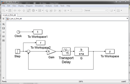
For example, the model below is an example of feedback with a first order transfer function and a delay. First in Simulink:
and now in xcos
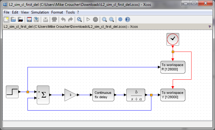
Part of the exercise set for the students is to define all of the relevant parameters in the workspace: b,a,k and so on. If you attempt to download and run the above, you’ll have to do that in order to make them work. You’ll also need extract and plot the results from the workspace.
It can be seen that the two models look very similar and, for these examples at least, it really doesn’t matter which piece of software the students use.
The full set of MATLAB/Simulink examples along with Danail’s Scilab/Xcos conversions can be found at http://personalpages.manchester.ac.uk/staff/William.Heath/matlab_scilab.html
Introduction
Mathematica 10 was released yesterday amid the usual marketing storm we’ve come to expect for a new product release from Wolfram Research. Some of the highlights of this marketing information include
- Mathematica 10 blog post by Stephen Wolfram
- What’s new in 10? From Wolfram Research
- Alphabetical list of new functions
Without a doubt, there is a lot of great new functionality in this release and I’ve been fortunate enough to have access to some pre-releases for a while now. There is no chance that I can compete with the in-depth treatments given by Wolfram Research of the 700+ new functions in Mathematica 10 so I won’t try. Instead, I’ll hop around some of the new features, settling on those that take my fancy.
Multiple Undo
I’ve been a Mathematica user since version 4 of the product which was released way back in 1999. For the intervening 15 years, one aspect of Mathematica that always frustrated me was the fact that the undo feature could only undo the most recent action. I, along with many other users, repeatedly asked for multiple undo to be implemented but were bitterly disappointed for release after release.
Few things have united Mathematica users more than the need for multiple undo:
- A website with petition calling for multiple undo
- A Facebook page calling for multiple undo
- A very popular Mathematica StackExchange question about multiple undo
Finally, with version 10, our hopes and dreams have been answered and multiple undo is finally here. To be perfectly honest, THIS is the biggest reason to upgrade to version 10. Everything else is just tasty gravy.
Key new areas of functionality
Most of the things considered in this article are whimsical and only scratch the surface of what’s new in Mathematica 10. I support Mathematica (and several other products) at the University of Manchester in the UK and so I tend to be interested in things that my users are interested in. Here’s a brief list of new functionality areas that I’ll be shouting about
- Machine Learning I know several people who are seriously into machine learning but few of them are Mathematica users. I’d love to know what they make of the things on offer here.
- New image processing functions The Image Processing Toolbox is one of the most popular MATLAB toolboxes on my site. I wonder if this will help turn MATLAB-heads. I also know people in a visualisation group who may be interested in the new 3D functions on offer.
- Nonlinear control theoryVarious people in our electrical engineering department are looking at alternatives to MATLAB for control theory. Maple/Maplesim and Scilab/Xcos are the key contenders. SystemModeler is too expensive for us to consider but the amount of control functionality built into Mathematica is useful.
Entities – a new data type for things that Mathematica knows stuff about
One of the new functions I’m excited about is GeoGraphics that pulls down map data from Wolfram’s servers and displays them in the notebook. Obviously, I did not read the manual and so my first attempt at getting a map of the United Kingdom was
GeoGraphics["United Kingdom"]
What I got was a map of my home town, Sheffield, surrounded by a red cell border indicating an error message
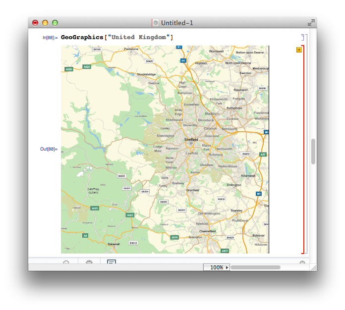
The error message is “United Kingdom is not a Graphics primitive or directive.” The practical upshot of this is that GeoGraphics is not built to take strings as arguments. Fair enough, but why the map of Sheffield? Well, if you call GeoGraphics[] on its own, the default action is to return a map centred on the GeoLocation found by considering your current IP address and it seems that it also does this if you send something bizarre to GeoGraphics. In all honesty, I’d have preferred no map and a simple error message.
In order to get what I want, I have to pass an Entity that represents the UK to the GeoGraphics function. Entities are a new data type in Mathematica 10 and, as far as I can tell, they formally represent ‘things’ that Mathematica knows about. There are several ways to create entities but here I use the new Interpreter function
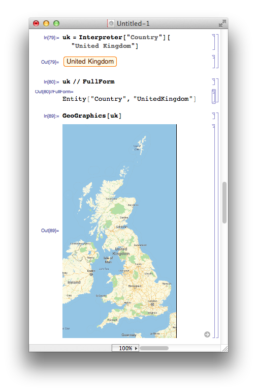
From the above, you can see that Entities have a special new StandardForm but their InputForm looks straightforward enough. One thing to bear in mind here is that all of the above functions require a live internet connection in order to work. For example, on thinking that I had gotten the hang of the Entity syntax, I switched off my internet connection and did
mycity = Entity["City", "Manchester"]

During evaluation of In[92]:= URLFetch::invhttp: Couldn't resolve host name. >>

During evaluation of In[92]:= WolframAlpha::conopen: Using WolframAlpha requires internet connectivity. Please check your network connection. You may need to configure your firewall program or set a proxy in the Internet Connectivity tab of the Preferences dialog. >>

Out[92]= Entity["City", "Manchester"]
So, you need an internet connection even to create entities at this most fundamental level. Perhaps it’s for validation? Turning the internet connection back on and re-running the above command removes the error message but the thing that’s returned isn’t in the new StandardForm:
![]()
If I attempt to display a map using the mycity variable, I get the map of Sheffield that I currently associate with something having gone wrong (If I’d tried this out at work,in Manchester, on the other hand, I would think it had worked perfectly!). So, there is something very wrong with the entity I am using here – It doesn’t look right and it doesn’t work right – clearly that connection to WolframAlpha during its creation was not to do with validation (or if it was, it hasn’t helped). I turn back to the Interpreter function:
In[102]:= mycity2 = Interpreter["City"]["Manchester"] // InputForm

Out[102]//InputForm:= Entity["City", {"Manchester", "Manchester", "UnitedKingdom"}]
So, clearly my guess at how a City entity should look was completely incorrect. For now, I think I’m going to avoid creating Entities directly and rely on the various helper functions such as Interpreter.
What are the limitations of knowledge based computation in Mathematica?
All of the computable data resides in the Wolfram Knowledgebase which is a new name for the data store used by Wolfram Alpha, Mathematica and many other Wolfram products. In his recent blog post, Stephen Wolfram says that they’ll soon release the Wolfram Discovery Platform which will allow large scale access to the Knowledgebase and indicated that ‘basic versions of Mathematica 10 are just set up for small-scale data access.’ I have no idea what this means and what limitations are in place and can’t find anything in the documentation.
Until I understand what limitations there might be, I find myself unwilling to use these data-centric functions for anything important.
IntervalSlider – a new control for Manipulate
I’ll never forget the first time I saw a Mathematica Manipulate – it was at the 2006 International Mathematica Symposium in Avignon when version 6 was still in beta. A Wolfram employee created a fully functional, interactive graphical user interface with just a few lines of code in about 2 minutes –I’d never seen anything like it and was seriously excited about the possibilities it represented.
8 years and 4 Mathematica versions later and we can see just how amazing this interactive functionality turned out to be. It forms the basis of the Wolfram Demonstrations project which currently has 9677 interactive demonstrations covering dozens of fields in engineering, mathematics and science.
Not long after Mathematica introduced Manipulate, the sage team introduced a similar function called interact. The interact function had something that Manipulate did not – an interval slider (see the interaction called ‘Numerical integrals with various rules’ at http://wiki.sagemath.org/interact/calculus for an example of it in use). This control allows the user to specify intervals on a single slider and is very useful in certain circumstances.
As of version 10, Mathematica has a similar control called an IntervalSlider. Here’s some example code of it in use
Manipulate[
 pl1 = Plot[Sin[x], {x, -Pi, Pi}];
 pl2 = Plot[Sin[x], {x, range[[1]], range[[2]]}, Filling -> Axis,
   PlotRange -> {-Pi, Pi}];
 inset = Inset["The Integral is approx " <> ToString[
     NumberForm[
      Integrate[Sin[x], {x, range[[1]], range[[2]]}]
      , {3, 3}, ExponentFunction -> (Null &)]], {2, -0.5}];
 Show[{pl1, pl2}, Epilog -> inset], {{range, {-1.57, 1.57}}, -3.14,
  3.14, ControlType -> IntervalSlider, Appearance -> "Labeled"}]
and here’s the result:

Associations – A new kind of brackets
Mathematica 10 brings a new fundamental data type to the language, associations. As far as I can tell, these are analogous to dictionaries in Python or Julia since they consist of key,value pairs. Since Mathematica has already used every bracket type there is, Wolfram Research have had to invent a new one for associations.
Let’s create an association called scores that links 3 people to their test results
In[1]:= scores = <|"Mike" -> 50.2, "Chris" -> 100.00, "Johnathan" -> 62.3|>

Out[1]= <|"Mike" -> 50.2, "Chris" -> 100., "Johnathan" -> 62.3|>
We can see that the Head of the scores object is Association
In[2]:= Head[scores]

Out[2]= Association
We can pull out a value by supplying a key. For example, let’s see what value is associated with “Mike”
In[3]:= scores["Mike"]

Out[3]= 50.2
All of the usual functions you expect to see for dictionary-type objects are there:-
In[4]:= Keys[scores]

Out[4]= {"Mike", "Chris", "Johnathan"}

In[5]:= Values[scores]

Out[5]= {50.2, 100., 62.3}

In[6]:= (*Show that the key "Bob" does not exist in scores*)
KeyExistsQ[scores, "Bob"]

Out[6]= False
If you ask for a key that does not exist this happens:
In[7]:= scores["Bob"]

Out[7]= Missing["KeyAbsent", "Bob"]
There’s a new function called Counts that takes a list and returns an association which counts the unique elements in the list:
In[8]:= Counts[{q, w, e, r, t, y, u, q, w, e}]

Out[8]= <|q -> 2, w -> 2, e -> 2, r -> 1, t -> 1, y -> 1, u -> 1|>
Let’s use this to find something out something interesting, such as the most used words in the classic text, Moby Dick
In[1]:= (*Import Moby Dick from Project gutenberg*)

MobyDick =
  Import["http://www.gutenberg.org/cache/epub/2701/pg2701.txt"];
(*Split into words*)
words = StringSplit[MobyDick];
(*Convert all words to lowercase*)

words = Map[ToLowerCase[#] &, words];
(*Create an association of words and corresponding word count*)

wordcounts = Counts[words];
(*Sort the association by key value*)

wordcounts = Sort[wordcounts, Greater];
(*Show the top 10*)
wordcounts[[1 ;; 10]]

Out[6]= <|"the" -> 14413, "of" -> 6668, "and" -> 6309, "a" -> 4658,
 "to" -> 4595, "in" -> 4116, "that" -> 2759, "his" -> 2485,
 "it" -> 1776, "with" -> 1750|>
All told, associations are a useful addition to the Mathematica language and I’m happy to see them included. Many existing functions have been updated to handle Associations making them a fundamental part of the language.
- How to make use of Associations? – a question from Mathematica Stack Exchange
s/Mathematica/Wolfram Language/g
I’ve been programming in Mathematica for well over a decade but the language is no longer called ‘Mathematica’, it’s now called ‘The Wolfram Language.’ I’ll not lie to you, this grates a little but I guess I’ll just have to get used to it. Flicking through the documentation, it seems that a global search and replace has happened and almost every occurrence of ‘Mathematica’ has been changed to ‘The Wolfram Language’
This is part of a huge marketing exercise for Wolfram Research and I guess that part of the reason for doing it is to shift the emphasis away from mathematics to general purpose programming. I wonder if this marketing push will increase the popularity of The Wolfram Language as measured by the TIOBE index? Neither ‘Mathematica’ or ‘The Wolfram Language’ is listed in the top 100 and last time I saw more detailed results had it at number 128.
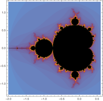
Fractal exploration
One of Mathematica’s competitors, Maple, had a new release recently which saw the inclusion of a set of fractal exploration functions. Although I found this a fun and interesting addition to the product, I did think it rather an odd thing to do. After all, if any software vendor is stuck for functionality to implement, there is a whole host of things to do that rank higher in most user’s list of priorities than a function that plots a standard fractal.
It seems, however, that both Maplesoft and Wolfram Research have seen a market for such functionality. Mathematica 10 comes with a set of functions for exploring the Mandelbrot and Julia sets. The Mandelbrot set alone accounts for at least 5 of Mathematica 10’s 700 new functions:- MandelbrotSetBoettcher, MandelbrotSetDistance, MandelbrotSetIterationCount, MandelbrotSetMemberQ and MandelbrotSetPlot.
MandelbrotSetPlot[]
Barcodes
I found this more fun than is reasonable! Mathematica can generate and recognize bar codes and QR codes in various formats. For example
BarcodeImage["www.walkingrandomly.com", "QR"]

Scanning the result using my mobile phone brings me right back home :)
Unit Testing
A decent unit testing framework is essential to anyone who’s planning to do serious software development. Python has had one for years, MATLAB got one in 2013a and now Mathematica has one. This is good news! I’ve not had chance to look at it in any detail, however. For now, I’ll simply nod in approval and send you to the documentation. Opinions welcomed.
Disappointments in Mathematica 10
There’s a lot to like in Mathematica 10 but there’s also several aspects that disappointed me
No update to RLink
Version 9 of Mathematica included integration with R which excited quite a few people I work with. Sadly, it seems that there has been no work on RLink at all between version 9 and 10. Issues include:
- The version of R bundled with RLink is stuck at 2.14.0 which is almost 3 years old. On Mac and Linux, it is not possible to use your own installation of R so we really are stuck with 2.14. On Windows, it is possible to use your own installation of R but CHECK THAT version 3 issue has been fixed http://mathematica.stackexchange.com/questions/27064/rlink-and-r-v3-0-1
- It is only possible to install extra R packages on Windows. Mac and Linux users are stuck with just base R.
This lack of work on RLink really is a shame since the original release was a very nice piece of work.
If the combination of R and notebook environment is something that interests you, I think that the current best solution is to use the R magics from within the IPython notebook.
No update to CUDA/OpenCL functions
Mathematica introduced OpenCL and CUDA functionality back in version 8 but very little appears to have been done in this area since. In contrast, MATLAB has improved on its CUDA functionality (it has never supported OpenCL) every release since its introduction in 2010b and is now superb!
Accelerating computations using GPUs is a big deal at the University of Manchester (my employer) which has a GPU-club made up of around 250 researchers. Sadly, I’ll have nothing to report at the next meeting as far as Mathematica is concerned.
FinancialData is broken (and this worries me more than you might expect)
I wrote some code a while ago that used the FinancialData function and it suddenly stopped working because of some issue with the underlying data source. In short, this happens:
In[12]:= FinancialData["^FTAS", "Members"]

Out[12]= Missing["NotAvailable"]
This wouldn’t be so bad if it were not for the fact that an example given in Mathematica’s own documentation fails in exactly the same way! The documentation in both version 9 and 10 give this example:
In[1]:= FinancialData["^DJI", "Members"]

Out[1]= {"AA", "AXP", "BA", "BAC", "CAT", "CSCO", "CVX", "DD", "DIS", \
"GE", "HD", "HPQ", "IBM", "INTC", "JNJ", "JPM", "KFT", "KO", "MCD", \
"MMM", "MRK", "MSFT", "PFE", "PG", "T", "TRV", "UTX", "VZ", "WMT", \
"XOM"}
but what you actually get is
In[1]:= FinancialData["^DJI", "Members"]

Out[1]= Missing["NotAvailable"]
For me, the implications of this bug are far more reaching than a few broken examples. Wolfram Research are making a big deal of the fact that Mathematica gives you access to computable data sets, data sets that you can just use in your code and not worry about the details.
Well, I did just as they suggest, and it broke!
Summary
I’ve had a lot of fun playing with Mathematica 10 but that’s all I’ve really done so far – play – something that’s probably obvious from my choice of topics in this article. Even through play, however, I can tell you that this is a very solid new release with some exciting new functionality. Old-time Mathematica users will want to upgrade for multiple-undo alone and people new to the system have an awful lot of toys to play with.
Looking to the future of the system, I feel excited and concerned in equal measure. There is so much new functionality on offer that it’s almost overwhelming and I love the fact that its all integrated into the core system. I’ve always been grateful of the fact that Mathematica hasn’t gone down the route of hiving functionality off into add-on products like MATLAB does with its numerous toolboxes.
My concerns center around the data and Stephen Wolfram’s comment ‘basic versions of Mathematica 10 are just set up for small-scale data access.’ What does this mean? What are the limitations and will this lead to serious users having to purchase add-ons that would effectively be data-toolboxes?
Final
Have you used Mathematica 10 yet? If so, what do you think of it? Any problems? What’s your favorite function?
Mathematica 10 links
- Playing with Mathematica on Raspberry Pi – The Raspberry Pi was the first platform that saw Mathematica version 10…and it’s free!
Something that became clear from my recent comparison of Numpy’s Mersenne Twister implementation with MATLAB’s is that there is something funky going on with seed 0 in MATLAB. A discussion in the comments thread helped uncover what was going on. In short, seed 0 gives exactly the same random numbers as seed 5489 in MATLAB (unless you use their deprecated rand(‘twister’,0) syntax).
This is a potential problem for anyone who performs lots of simulations that make use of random numbers such as monte-carlo simulations. One common work-flow is to run the same program hundreds of times where only the seed differs between runs. This is probably good enough to ensure that each simulation uses a random number stream that is statistically independent from all of the others — There is a risk that some streams will overlap but the probability is low and most people are content to live with that risk.
The practical upshot of this is that if you intend on sticking with Mersenne Twister for your MATLAB monte-carlo simulations, it might be wise to avoid seed 0. Alternatively, move to a random number generator that guarantees non-overlapping, independent streams – something that any implementation of Mersenne Twister cannot do.
Here’s a demo run in MATLAB 2014a on Windows 7.
>> format long
>> rng(0)
>> rand(1,5)'

ans =

   0.814723686393179
   0.905791937075619
   0.126986816293506
   0.913375856139019
   0.632359246225410

>> rng(5489)
>> rand(1,5)'

ans =

   0.814723686393179
   0.905791937075619
   0.126986816293506
   0.913375856139019
   0.632359246225410
When porting code between MATLAB and Python, it is sometimes useful to produce the exact same set of random numbers for testing purposes. Both Python and MATLAB currently use the Mersenne Twister generator by default so one assumes this should be easy…and it is…provided you use the generator in Numpy and avoid the seed 0.
Generate some random numbers in MATLAB
Here, we generate the first 5 numbers for 3 different seeds in MATLAB. Our aim is to reproduce these in Python.
>> format long
>> rng(0)
>> rand(1,5)'

ans =

   0.814723686393179
   0.905791937075619
   0.126986816293506
   0.913375856139019
   0.632359246225410

>> rng(1)
>> rand(1,5)'

ans =

   0.417022004702574
   0.720324493442158
   0.000114374817345
   0.302332572631840
   0.146755890817113

>> rng(2)
>> rand(1,5)'

ans =

   0.435994902142004
   0.025926231827891
   0.549662477878709
   0.435322392618277
   0.420367802087489
Python’s default random module
According to the documentation,Python’s random module uses the Mersenne Twister algorithm but the implementation seems to be different from MATLAB’s since the results are different. Here’s the output from a fresh ipython session:
In [1]: import random

In [2]: random.seed(0)

In [3]: [random.random() for _ in range(5)]
Out[3]:
[0.8444218515250481,
 0.7579544029403025,
 0.420571580830845,
 0.25891675029296335,
 0.5112747213686085]

In [4]: random.seed(1)

In [5]: [random.random() for _ in range(5)]
Out[5]:
[0.13436424411240122,
 0.8474337369372327,
 0.763774618976614,
 0.2550690257394217,
 0.49543508709194095]

In [6]: random.seed(2)

In [7]: [random.random() for _ in range(5)]
Out[7]:
[0.9560342718892494,
 0.9478274870593494,
 0.05655136772680869,
 0.08487199515892163,
 0.8354988781294496]
The Numpy random module
Numpy’s random module, on the other hand, seems to use an identical implementation to MATLAB for seeds other than 0. In the below, notice that for seeds 1 and 2, the results are identical to MATLAB’s. For a seed of zero, they are different.
In [1]: import numpy as np

In [2]: np.set_printoptions(suppress=True)

In [3]: np.set_printoptions(precision=15)

In [4]: np.random.seed(0)

In [5]: np.random.random((5,1))
Out[5]:
array([[ 0.548813503927325],
       [ 0.715189366372419],
       [ 0.602763376071644],
       [ 0.544883182996897],
       [ 0.423654799338905]])

In [6]: np.random.seed(1)

In [7]: np.random.random((5,1))
Out[7]:
array([[ 0.417022004702574],
       [ 0.720324493442158],
       [ 0.000114374817345],
       [ 0.30233257263184 ],
       [ 0.146755890817113]])

In [8]: np.random.seed(2)

In [9]: np.random.random((5,1))
Out[9]:
array([[ 0.435994902142004],
       [ 0.025926231827891],
       [ 0.549662477878709],
       [ 0.435322392618277],
       [ 0.420367802087489]])
Checking a lot more seeds
Although the above interactive experiments look convincing, I wanted to check a few more seeds. All seeds from 0 to 1 million would be a good start so I wrote a MATLAB script that generated 10 random numbers for each seed from 0 to 1 million and saved the results as a .mat file.
A subsequent Python script loads the .mat file and ensures that numpy generates the same set of numbers for each seed. It outputs every seed for which Python and MATLAB differ.
On my mac, I opened a bash prompt and ran the two scripts as follows
matlab -nodisplay -nodesktop -r "generate_matlab_randoms"
python python_randoms.py
The output was
MATLAB file contains 1000001 seeds and 10 samples per seed
Random numbers for seed 0 differ between MATLAB and Numpy
System details
- Late 2013 Macbook Air
- MATLAB 2014a
- Python 2.7.7
- Numpy 1.8.1
One of my favourite MATLAB books is The MATLAB Guide by Desmond and Nicholas Higham. The first chapter, called ‘A Brief Tutorial’ shows how various mathematical problems can be easily explored with MATLAB; things like continued fractions, random fibonacci sequences, fractals and collatz iterations.
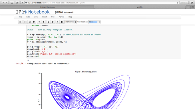
Over at the SIAM blog, Don MacMillen, demonstrates how its now possible, trivial even, to rewrite the entire chapter as an IPython notebook with all MATLAB code replaced with Python.
The notebook is available as a gist and can be viewed statically on nbviewer.
What other examples of successful MATLAB->Python conversions have you found?
If you’ve ever wanted to use MATLAB to develop personal projects or as a hobby but have been put off by the eye-watering commercial prices, the new MATLAB Home edition might be for you.
For £85 you get full powered MATLAB without any toolboxes. This is the same version that the professionals use but there are various restrictions on its use. The FAQ states “The MATLAB® Home license is for your personal use only. It is not available for government, academic, research, commercial, or other organizational use.”
It is possible to buy toolboxes for an extra £25 each but, at the time of writing at least, it is not possible to buy ALL available toolboxes on the home license.
Some of Mathworks’ competitors have had similar home-use licenses available for some time – Mathematica and Maple to name two – it’s great to see MATLAB added to this list.
Other WalkingRandomly posts you may be interested in