Walking Randomly

The test suite of a project I’m working on is poking around at the extreme edges of the range of double precision numbers. I noticed a difference between Windows and other platforms that I can’t yet fully explain. On Windows, the test suite was pumping out RuntimeWarnings that we don’t see in Linux or Mac. I’ve distilled the issue down to a single numpy command:

np.log1p(1.7976931348622732e+308)

On Windows 7 Anaconda Python 2.3, this gives a RuntimeWarning and returns inf whereas on Linux and Mac OS X it evaluates to 709.78-ish

Numpy version is 1.9.2 in all cases.

64 bit Windows 7

Python 2.7.10 |Continuum Analytics, Inc.| (default, May 28 2015, 16:44:52) [MSC
v.1500 64 bit (AMD64)] on win32
Type "help", "copyright", "credits" or "license" for more information.
Anaconda is brought to you by Continuum Analytics.
Please check out: http://continuum.io/thanks and https://binstar.org
>>> import numpy as np
>>> np.log1p(1.7976931348622732e+308)
__main__:1: RuntimeWarning: overflow encountered in log1p
inf

64 bit Linux

Python 2.7.9 (default, Apr  2 2015, 15:33:21) 
[GCC 4.9.2] on linux2
Type "help", "copyright", "credits" or "license" for more information.
>>> import numpy as np
>>> np.log1p(1.7976931348622732e+308)
709.78271289338397

Mac OS X

Python 2.7.10 |Anaconda 2.3.0 (x86_64)| (default, May 28 2015, 17:04:42) 
[GCC 4.2.1 (Apple Inc. build 5577)] on darwin
Type "help", "copyright", "credits" or "license" for more information.
Anaconda is brought to you by Continuum Analytics.
Please check out: http://continuum.io/thanks and https://binstar.org
>>> import numpy as np
>>> np.log1p(1.7976931348622732e+308)
709.78271289338397

The argument to log1p is getting close to the largest double precision number:

>>> sys.float_info.max
1.7976931348623157e+308

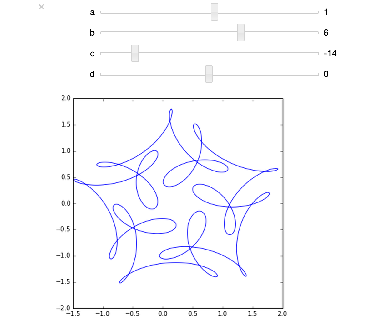
The ever-superb John D. Cook recently found this lovely looking curve in a book he’s currently reading

John posted some Python code that reproduced this curve. I stole borrowed his code, put it in a Jupyter notebook and wrapped it in an interactive widget to allow me to play with the parameters and see what other curves I could come up with. The result looks like this.

If you’d like something where those sliders work, you need to run the notebook I’ve created in Project Jupyter. Here are 2 ways to do that.

• Download the notebook from github
• Method 1: Upload this notebook to Try Jupyter.
• Method 2: Install Anaconda Python on your machine. Launch the notebook and open the file downloaded above.

Once you have the notebook open, click on Cell->Run All and play with the sliders that pop up.

Other posts about these curves:

• Random cyclic curves – Includes code written in Haskell
• A geogebra applet

I recently found myself in need of a portable install of the Jupyter notebook which made use of a portable install of R as the compute kernel. When you work in institutions that have locked-down managed Windows desktops, such portable installs can be a life-saver! This is particularly true when you are working with rapidly developing projects such as Jupyter and IRKernel.

It’s not perfect but it works for the fairly modest requirements I had for it. Here are the steps I took to get it working.

Download and install Portable Python

I downloaded Portable Python 2.7.6.1 from http://portablepython.com/ and installed into a directory called Portable Python 2.7.6.1

Update IPython and install the extra modules we need

This version of Portable Python comes with a portable IPython instance but it is too old to support alternative kernels. As such, we need to install a newer version.

Open a cmd.exe command prompt and navigate to Portable Python 2.7.6.1\App\Scripts.

Enter the command

easy_install ipython.exe

You’ll now find that you can launch the ipython.exe terminal from within this directory:

C:\Users\walkingrandomly\Desktop\Portable Python 2.7.6.1\App\Scripts>ipython
Python 2.7.6 (default, Nov 10 2013, 19:24:18) [MSC v.1500 32 bit (Intel)]
Type "copyright", "credits" or "license" for more information.

IPython 3.1.0 -- An enhanced Interactive Python.
?         -> Introduction and overview of IPython's features.
%quickref -> Quick reference.
help      -> Python's own help system.
object?   -> Details about 'object', use 'object??' for extra details.

In [1]: exit()

If you try to launch the notebook, however, you’ll get error messages. This is because we haven’t taken care of all the dependencies. Let’s do that now. Ensuring you are still in the Portable Python 2.7.6.1\App\Scripts folder, execute the following commands.

easy_install pyzmq
easy_install jinja2
easy_install tornado
easy_install jsonschema

You should now be able to launch the notebook using

ipython notebook

Install portable R and IRKernel

• I downloaded Portable R 3.2 from http://sourceforge.net/projects/rportable/files/ and installed into a directory called R-Portable
• Move this directory into the Portable Python directory. It needs to go inside Portable Python 2.7.6.1\App (see this discussion to learn how I discovered that this location was the correct one)
• Launch the Portable R executable which should be at Portable Python 2.7.6.1\App\R-Portable\R-portable.exe and install the IRKernel packages by doing

install.packages(c("rzmq","repr","IRkernel","IRdisplay"), repos="http://irkernel.github.io/")

Install additional R packages

The version of Portable R I used didn’t include various necessary packages. Here’s how I fixed that.

• Launch the Portable R executable which should be at Portable Python 2.7.6.1\App\R-Portable\R-portable.exe and install the following packages 

  install.packages('digest')
  install.packages('uuid')
  install.packages('base64enc')
  install.packages('evaluate')
  install.packages('jsonlite')

Install the R kernel file
Create the directory structure Portable Python 2.7.6.1\App\share\jupyter\kernels\R_kernel

Create a file called kernel.json that contains the following

{"argv": ["R-Portable/App/R-Portable/bin/i386/R.exe","-e","IRkernel::main()",
"--args","{connection_file}"],
 "display_name":"Portable R"
}

This file needs to go in the R_kernel directory created earlier. Note that the kernel location specified in kernel.json uses Linux style forward slashes in the path rather than the backslashes that Windows users are used to. I found that this was necessary for the kernel to work –it was ignored by the notebook otherwise.

Finishing off

Everything created so far, including R, is in the folder Portable Python 2.7.6

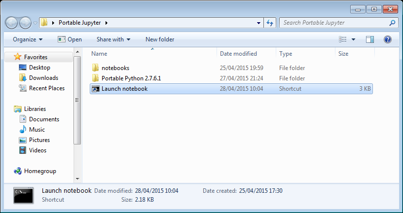
I created a folder called PortableJupyter and put the Portable Python 2.7.6 folder inside it. I also created the folder PortableJupyter\notebooks to allow me to carry my notebooks around with the software that runs them.

There is a bug in Portable Python 2.7.6.1 relating to scripts like IPython.exe that have been installed using easy_install. In short, they stop working if you move the directory they’re installed in – breaking portability somewhat! (Details here)

The workaround is to launch Ipython by running the script Portable Python 2.7.6.1\App\Scripts\ipython-script.py

I didn’t want to bother with that so created a shortcut in my PortableJupyter folder called Launch notebook. The target of this shortcut was the following line

%windir%\system32\cmd.exe /c "cd notebooks && "%CD%/Portable Python 2.7.6.1/App\python.exe" "%CD%/Portable Python 2.7.6.1\App\Scripts\ipython-script.py" notebook"

This starts the notebook using the default web browser and puts you in the notebooks directory.

The pay off

My folder looks like this:

If I click on the Launch Notebook shortcut, I get a Jupyter session with 2 kernel options

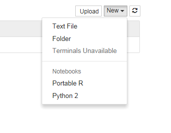
I can choose the Portable R kernel and start using R in the notebook!

If you really want to learn the differences between Python 2 and Python 3, I suggest you try converting a non-trivial software project. I’m in the middle of doing one now and am learning all kinds of little gotchas over and above the standard stuff that everyone knows such as changes to print, integer division and removal of xrange.

The most recent one I learned about (about 10 minutes ago) amounted to this

#Python 2.7.6 (default, Mar 22 2014, 22:59:56) 
[GCC 4.8.2] on linux2
Type "help", "copyright", "credits" or "license" for more information.
>>> [x for x in range(10)]
[0, 1, 2, 3, 4, 5, 6, 7, 8, 9]
>>> x
9

compared to

Python 3.4.0 (default, Apr 11 2014, 13:05:11) 
[GCC 4.8.2] on linux
Type "help", "copyright", "credits" or "license" for more information.
>>> [x for x in range(10)]
[0, 1, 2, 3, 4, 5, 6, 7, 8, 9]
>>> x
Traceback (most recent call last):
  File "", line 1, in 
NameError: name 'x' is not defined

This is well documented (This StackOverflow Q+A is great!) but I didn’t know about it and, in the code I was looking at, there was a heck of a lot of complication between the list comprehension and when ‘x’ was used. As such, it took me a while to figure out!

Another change that had me scratching my head for a while is the fact that Python 3 ignores the __metaclass__ hook. I didn’t know this little fact but discovered it while debugging failing tests!

Of course, once you know these little gotchas, you’ll probably not be caught out by them again in your next Python 2->Python 3 porting project but they got me wondering…..

What changes from Python 2->Python 3 have really caught you out at some point?

Linear Algebra – Foundations to Frontiers (or LAFF to its friends) is a popular, high quality and free MOOC that, as the title suggests, teaches aspects of linear algebra in a way that takes the student from the very basics through to some cutting edge techniques. I worked through much of it last year and thoroughly enjoyed the approach it took — focusing on programming aspects from the very beginning. The course authors are also among the developers of the FLAME project, a high performance linear algebra library, and one of the interesting aspects of the LAFF course (for me at least) was that it taught linear algebra in a way that also allowed you to understand the approaches used in the algorithms behind FLAME.

Last year, all of the programming assignments in LAFF were done in Python, making use of the IPython notebook. This year, the software stack will be different and will be based on MATLAB. I understand that everyone who signs up to LAFF will be able to get a free MATLAB license from Mathworks for the duration of the course. Understandably, this caused quite a bit of discussion between the LAFF team and software/language geeks like me. In a recent Facebook thread, I asked about the switch and received the reply

‘MATLAB will be free during the course. There are open source equivalents, but Mathworks staff is supporting the use of MATLAB (staff for us). There were some who never got the IPython notebooks to work properly. We are really excited at the opportunity to innovate again and perhaps clear up snags in the programming issues we had. It was complicated to support IPython on all of the operating systems and machines that participants use. MATLAB promises to be easier and will allow us again to concentrate on the Linear Algebra’ – LAFF UTx

I’m sufficiently interested in this change from IPython to MATLAB that I’ll be signing up for the course again this year and I encourage you to do the same — I believe that the programming-centric teaching approach taken by LAFF is extremely well done and your time would be well-spent working through the course.

The course starts on 28th January 2015 so sign up now!

Here’s the trailer for last year’s course.

Given a symmetric matrix such as

What’s the nearest correlation matrix? A 2002 paper by Manchester University’s Nick Higham which answered this question has turned out to be rather popular! At the time of writing, Google tells me that it’s been cited 394 times.

Last year, Nick wrote a blog post about the algorithm he used and included some MATLAB code. He also included links to applications of this algorithm and implementations of various NCM algorithms in languages such as MATLAB, R and SAS as well as details of the superb commercial implementation by The Numerical algorithms group.

I noticed that there was no Python implementation of Nick’s code so I ported it myself.

Here’s an example IPython session using the module

In [1]: from nearest_correlation import nearcorr

In [2]: import numpy as np

In [3]: A = np.array([[2, -1, 0, 0], 
   ...:               [-1, 2, -1, 0],
   ...:               [0, -1, 2, -1], 
   ...:               [0, 0, -1, 2]])

In [4]: X = nearcorr(A)

In [5]: X
Out[5]: 
array([[ 1.        , -0.8084125 ,  0.1915875 ,  0.10677505],
       [-0.8084125 ,  1.        , -0.65623269,  0.1915875 ],
       [ 0.1915875 , -0.65623269,  1.        , -0.8084125 ],
       [ 0.10677505,  0.1915875 , -0.8084125 ,  1.        ]])

This module is in the early stages and there is a lot of work to be done. For example, I’d like to include a lot more examples in the test suite, add support for the commercial routines from NAG and implement other algorithms such as the one by Qi and Sun among other things.

Hopefully, however, it is just good enough to be useful to someone. Help yourself and let me know if there are any problems. Thanks to Vedran Sego for many useful comments and suggestions.

• github repository for the Python NCM module, nearest_correlation
• Nick Higham’s original MATLAB code.
• NAG’s commercial implementation – callable from C, Fortran, MATLAB, Python and more. A superb implementation that is significantly faster and more robust than this one!

The Mathematics department at The University of Manchester runs a third year undergraduate module called ‘Problem solving by computer’ which invites students to solve complex mathematical problems by doing a little programming. Along with some interesting mathematics, the course exposes students to a wide variety of languages and numerical libraries including MATLAB, Octave, NAG, Mathematica and, most recently, Python.

Earlier this year, Python was introduced as an option for students who wanted to use it for a project in this course and, despite only being given two lectures in the language, quite a few people chose to use it. Much of this success must be attributed to the Python for MATLABers notes written by Manchester PhD student, Sophia Coban which is why I’m providing links to them here.

• Python for MATLAB users
• Numpy and Scipy for MATLAB users

When porting code between MATLAB and Python, it is sometimes useful to produce the exact same set of random numbers for testing purposes.  Both Python and MATLAB currently use the Mersenne Twister generator by default so one assumes this should be easy…and it is…provided you use the generator in Numpy and avoid the seed 0.

Generate some random numbers in MATLAB

Here, we generate the first 5 numbers for 3 different seeds in MATLAB. Our aim is to reproduce these in Python.

>> format long
>> rng(0)
>> rand(1,5)'

ans =

   0.814723686393179
   0.905791937075619
   0.126986816293506
   0.913375856139019
   0.632359246225410

>> rng(1)
>> rand(1,5)'

ans =

   0.417022004702574
   0.720324493442158
   0.000114374817345
   0.302332572631840
   0.146755890817113

>> rng(2)
>> rand(1,5)'

ans =

   0.435994902142004
   0.025926231827891
   0.549662477878709
   0.435322392618277
   0.420367802087489

Python’s default random module

According to the documentation,Python’s random module uses the Mersenne Twister algorithm but the implementation seems to be different from MATLAB’s since the results are different.  Here’s the output from a fresh ipython session:

In [1]: import random

In [2]: random.seed(0)

In [3]: [random.random() for _ in range(5)]
Out[3]: 
[0.8444218515250481,
 0.7579544029403025,
 0.420571580830845,
 0.25891675029296335,
 0.5112747213686085]

In [4]: random.seed(1)

In [5]: [random.random() for _ in range(5)]
Out[5]: 
[0.13436424411240122,
 0.8474337369372327,
 0.763774618976614,
 0.2550690257394217,
 0.49543508709194095]

In [6]: random.seed(2)

In [7]: [random.random() for _ in range(5)]
Out[7]: 
[0.9560342718892494,
 0.9478274870593494,
 0.05655136772680869,
 0.08487199515892163,
 0.8354988781294496]

The Numpy random module

Numpy’s random module, on the other hand, seems to use an identical implementation to MATLAB for seeds other than 0. In the below, notice that for seeds 1 and 2, the results are identical to MATLAB’s. For a seed of zero, they are different.

In [1]: import numpy as np

In [2]: np.set_printoptions(suppress=True)

In [3]: np.set_printoptions(precision=15)

In [4]: np.random.seed(0)

In [5]: np.random.random((5,1))
Out[5]: 
array([[ 0.548813503927325],
       [ 0.715189366372419],
       [ 0.602763376071644],
       [ 0.544883182996897],
       [ 0.423654799338905]])

In [6]: np.random.seed(1)

In [7]: np.random.random((5,1))
Out[7]: 
array([[ 0.417022004702574],
       [ 0.720324493442158],
       [ 0.000114374817345],
       [ 0.30233257263184 ],
       [ 0.146755890817113]])

In [8]: np.random.seed(2)

In [9]: np.random.random((5,1))
Out[9]: 
array([[ 0.435994902142004],
       [ 0.025926231827891],
       [ 0.549662477878709],
       [ 0.435322392618277],
       [ 0.420367802087489]])

Checking a lot more seeds

Although the above interactive experiments look convincing, I wanted to check a few more seeds. All seeds from 0 to 1 million would be a good start so I wrote a MATLAB script that generated 10 random numbers for each seed from 0 to 1 million and saved the results as a .mat file.

A subsequent Python script loads the .mat file and ensures that numpy generates the same set of numbers for each seed. It outputs every seed for which Python and MATLAB differ.

• generate_matlab_randoms.m
• python_randoms.py

On my mac, I opened a bash prompt and ran the two scripts as follows

matlab -nodisplay -nodesktop -r "generate_matlab_randoms"
python python_randoms.py

The output was

MATLAB file contains 1000001 seeds and 10 samples per seed
Random numbers for seed 0 differ between MATLAB and Numpy

System details

• Late 2013 Macbook Air
• MATLAB 2014a
• Python 2.7.7
• Numpy 1.8.1

One of my favourite MATLAB books is The MATLAB Guide by Desmond and Nicholas Higham. The first chapter, called ‘A Brief Tutorial’ shows how various mathematical problems can be easily explored with MATLAB; things like continued fractions, random fibonacci sequences, fractals and collatz iterations.

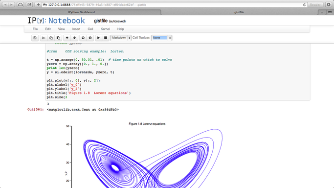
Over at the SIAM blog, Don MacMillen, demonstrates how its now possible, trivial even, to rewrite the entire chapter as an IPython notebook with all MATLAB code replaced with Python.

The notebook is available as a gist and can be viewed statically on nbviewer.

What other examples of successful MATLAB->Python conversions have you found?

The IPython project started as a procrastination task for Fernando Perez during his PhD and is currently one of the most exciting and important pieces of software in computational science today. Last month, Fernando joined us at The University of Manchester after being invited by Nick Higham of the department of Mathematics under the auspices of the EPSRC Network Numerical Algorithms and High Performance Computing

While at Manchester, Fernando gave a couple of talks and we captured one of them using the University of Manchester Lecture Podcasting Service (itself based on a Python project). Check it out below.