Walking Randomly

Right now we are all being subjected to some pretty depressing news. Flicking through today’s newspaper I see article after article on things like the credit crunch, the global energy crisis and impending recession. In the face of all this doom and gloom what we need is as many excuses to celebrate as possible.

Birthdays are a great excuse for celebration – a night out (or in) with friends, good food and maybe a glass (or three) of wine but the problem with birthdays is that they only come around once a year. Once a year, that is, if you only consider Earthly years but if you expand the net to include Martian years, Jovian years and, best of all, Mercurian years then you get a whole new set of celebration dates for your calendar.

The problem you are now faced with is working out when your next Martian birthday is. That’s where this Wolfram Demonstration from Chris Boucher comes in handy. Simply enter your birthdate and you’ll instantly get told your age as it would be on the various planets of the solar system. Despite it’s recent demotion from planetary status, Pluto has been included as well, and rightly so in my opinion. As an added bonus you’ll get told when your next birthday will be on each planet – helping you to fill up that all important celebration calendar. Cheers!

If you enjoyed this article, feel free to click here to subscribe to my RSS Feed.

One of the great things about the Wolfram Demonstrations Project is the fact that source code is included. This means that it is straightforward to take someone else’s code, learn how it works and then maybe tweak it to suit yourself. Back in February I did exactly that and used the code in Enrique Zeleny‘s Tangram puzzle as the basis for my own Valentine’s day version – The Broken Heart Tangram puzzle.

Things move on though and another demonstrations author, Karl Scherer has produced his own versions of both the Broken Heart and the Traditional tangram puzzles. Karl’s versions are faster, sleeker and generally more fun to use. As an added bonus I get to look at the source code to see how he did it – everyone’s a winner!

“Do you like pendulums?” I was asked, “because if you don’t like pendulums then I wouldn’t bother with A-Level physics if I were you.” This was the advice given to me by an outgoing sixth-former at a school open day around 14 years ago. He had obviously had an unhappy time during his physics studies and was doing his best to turn me away from the subject but he hadn’t counted on the fact that I actually do like pendulums. Besides, I figured that high-school physics isn’t only about pendulums – they’ve got springs too!

Of course everyone knows what a pendulum is – thing that swings back and forth, used in grandfather clocks. When all is said and done, you might argue that pendulums are simple, sometimes useful and, above all, dull. My sixth-form friend certainly thought so but maybe that was because he didn’t have enough pendulums!

One pendulum is useful but two are much more interesting and four can be downright fun! The Victorians certainly thought so and over 100 years ago they used to build home entertainment devices out of pendulums called harmonographs. You have probably never heard of a harmonograph (I certainly hadn’t until a couple of days ago) and so maybe a bit of detailed explanation is in order.

Imagine that you have attached a pencil to a pendulum so that it brushes across a piece of paper as the pendulum swings back and forth. When the pendulum finishes swinging you will end up with a single straight line drawn on your paper – very dull indeed! Now imagine further that you somehow manage to connect a second pendulum to your pencil which oscillates at right angles to the first. The resulting drawing might look something like the image below. If your imagination fails you (or if my explanation isn’t up to the job) then you can see a video of the set up I am trying to describe by clicking here.

Alternatively, you could have one pendulum attached to the pencil and another attached to the drawing surface as in the example below.

There are many different designs for harmonographs and some manage to incorporate up to 4 different independent oscillations by attaching pendulums to the drawing surface as well as the pencil itself. The resulting drawings can be spectacular.

So how might we go about simulating a harmonograph? Well the motion of a single damped pendulum along the x axis can be described by the parametric equation

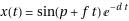
where t denotes time, p is a phase factor between 0 and 2*pi and d is the strength of the damping term. The larger you make d, the more quickly the pendulum oscillations will decay.

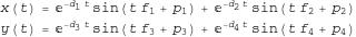
If we have two independent pendulums oscillating along the x-axis, both contributing to the overall motion of our pencil then, thanks to the principle of superposition, the total motion along the x-axis is given by

If we also have two pendulums oscillating along the y-axis then the final set of equations is

Now, if you search the internet you will find that other people have written down equations for harmonograph plots and you might find that they look slightly different to the ones I have written above but you should always be available to transform my equations into any other valid set. For example, the equations given in the website here describe a system with only three pendulums so simply cross out the second term for y(t) in my set of equations and you are almost done. You might also find that some people use Cosine instead of Sine – in which case you simply set the phase in my equations to be pi/2 since sin(x+pi/2) = cos(x).

Something else I have done is to assume that the initial amplitude of all of my pendulums is set to one. This is because I already have 12 parameters to play with which I think is more than enough for an initial play around.

As an aside, it turns out that these equations can describe much more than just Harmonographs. For example, by setting the damping factors to 0 and by crossing out the second term in each equation (thus only considering 2 oscillators) you will end up with Lissajous figures. With a bit of algebraic manipulation you can also obtain the equations that describe spirograph curves – see this link for the details.

So, we have a set of parametric equations and we want to plot the result. In Mathematica the ParametricPlot command is what we need so let’s give our 12 parameters some numbers and see what we can come up with.

ParametricPlot[{Sin[2 t + Pi/16] Exp[- 0.02 t] + Sin[6 t + 3 Pi/2] Exp[-0.0315 t], Sin[1.002 t + 13 Pi/16] Exp[-0.02 t] + Sin[3 t + Pi] Exp[-0.02 t]}, {t, 0, 167}, PlotRange -> All, Axes -> None]

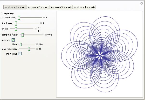
This is all very nice but it would be much nicer if we could manipulate the parameters with a set of sliders rather than having to manually type them in each time. My first attempt at producing such a graphical user interface to the above function in Mathematica looked like this (click the image to download an interactive notebook version that can be used in the free Mathematica Player application from Wolfram)

I quite like this version as you can see all of the parameters at once but it turned out to be too big for inclusion in the Wolfram Demonstrations Project. I tried various tricks to try and shoe-horn all of those parameters into a smaller applet and was about to give up when an employee at Wolfram sent me some code that sorted out the size problem by introducing a set of tabs. I like his solution so much that I’ll probably be writing about it soon in a separate article. The resulting Wolfram Demonstration was published today – click on the image below if you’d like to take a look.

Things that I haven’t done yet but might in the future include

• Animate the plot so that it looks more like the real thing.
• Add colour.
• Add the ability to modify the starting amplitude of each pendulum.

Of course the source code is available so if you have a burning desire to do any of these yourself then feel free – but please let me know if you do. I hope that you enjoy the results of these applets and would love to see any particularly interesting images that you might come up with – sending the equation parameters would be useful as well.
Parameters for reproducing the images above

Hover your mouse over a plot to see what image number it is

• Image 1: f₁=3.001 f₂=2 f₃=3 f₄=2 d₁=0.004 d₂=0.0065 d₃=0.008 d₄=0.019 p₁=0 p₂=0 p₃=pi/2 p₄=3pi/2
• Image 2: f₁=10 f₂=3 f₃=1 f₄=2 d₁=0.039 d₂=0.006 d₃=0 d₄=0.0045 p₁=0 p₂=0 p₃=pi/2 p₄=0
• Image 3: f₁=2.01 f₂=3 f₃=3 f₄=2 d₁=0.0085 d₂=0 d₃=0.065 d₄=0 p₁=0 p₂=7 pi/16 p₃=0 p₄=0
• Image 4: f₁=2 f₂=6 f₃=1.002 f₄=3 d₁=0.02 d₂=0.0315 d₃=0.02 d₄=0.02 p₁=pi/16 p₂=3pi/2 p₃=13 pi/16 p₄=pi

Harmonograph Resources

Hopefully, this article has whetted your appetite for harmonographs – if so then you might find the following resources interesting.

• How to Make a Three-Pendulum Rotary Harmonograph by Karl Sims
• Instructions for building your own harmonograph from chestofbooks.com
• More instructions for making harmonographs from 1920-30.com.
• Analysis of a home built harmonograph – a great model, I’m not sure about his equations though.
• Harmonograph – A visual guide to the Mathematics of Music. A book by Anthony Ashton.
• The Meccano Super Models (Volume 2) by Geoff Wright. ISBN 0-904568-07-5 contains instructions for making a Harmonograph out of Meccano. I can’t get hold of a copy unfortunately.
• The following two journal articles contains some interesting historical and technical information concerning harmonographs.
  • American Journal of Physics — February 2001 — Volume 69, Issue 2, pp. 162-173
  • American Journal of Physics — February 2001 — Volume 69, Issue 2, pp. 174-183
• Harmonograph simulator written in tcl.
• Java Harmonograph simulator.

If you enjoyed this article, feel free to click here to subscribe to my RSS Feed.

The Wolfram Demonstrations site has had something of a makeover and I think it looks great – definitely worth checking out if you have not been there for a while. If you are new here and haven’t heard about the Wolfram Demonstrations site then feel free to browse around Walking Randomly to see what I have written about it in the past. Alternatively you might care to head over there and see what it’s all about for yourself.

There are over 3500 different demonstrations available now – all of which can be downloaded and played with for free using Wolfram’s Mathematica Player. With everything from Spirographs through to Quantum Mechanics you will not fail to find something that interests you. I have got a few ideas swirling around my head at the moment so expect to see a few more from me soon (I also take requests by the way).

The only thing that really spoils the new site is the little picture of me that is currently under the ‘Featured Contributors’ section ;)

This is just a very quick post to highlight an idea from Maria over at the Teaching College Math Technology Blog. I agree with her, an application like spectra would be a cool way to browse the Wolfram Demonstrations Project. It would be even cooler if the user could control their posiiton in the cloud more directly though.

Many years ago (way WAY before the web), at the tender age of 10, I did a school math project about the Fibonacci numbers and got rather carried away with writing about the many different areas of mathematics and everyday life where this sequence popped up. Although I didn’t have the internet to help with my research, I did have a wonderful maths teacher called Ron Billington who taught for many years at Birchensale Middle School in Redditch. Mr Billington had a personal library of maths books that he collected over the years which was a treasure trove of material for someone like me who had significantly more enthusiasm than talent. He would have loved hearing about the little discovery I made while browsing through The College Mathematics Journal the other day.

First, a bit of background. The Fibonacci sequence starts off like this:

1 1 2 3 5 8 13 21

Each term in the sequence is formed from the sum of it’s two predecessors so the next term would be 13 + 21 = 34. What fascinated me as a child (and continues to fascinate me now) is the fact that this incredibly simple sequence of numbers, and others like it, seems to appear all over the place from the distribution of sunflower seeds to the study of photonic crystals.

There really is an astonishing amount of mathematics around the Fibonacci sequence as you will be able to verify with a quick google search. There is even an academic journal dedicated to the mathematics around it – The Fibonacci Quarterly – which I, unfortunately, have no access to at the moment (might have to have a word with the University librarian about that).

In the article Fibonacci Determinants, by Nathan Cahill et al (The College Mathematics Journal vol33 p221-225), the authors demonstrate the fact that you can obtain the nth term in the Fibonacci sequence by taking the determinant of a n x n tridiagonal matrix of the form

What’s more, if you change just a single entry (row 2 col 2) from 1 to 2 then you will obtain the Lucas Numbers instead. I thought that this was fun and so knocked up a Wolfram Demonstration for it which you can get to by clicking on the image below.

So Mr Billington – I have found yet another branch of Mathematics where the Fibonacci numbers turn up – Linear Algebra. I know it’s been 20 years but is there any chance of upping that B- to an A :) ?

If you enjoyed this article, feel free to click here to subscribe to my RSS Feed.

In the recent 30th edition of the Carnival of Mathematics, the author mentioned that 30 is the first Sphenic number. I had never heard the term before so I thought I would investigate them a bit – nothing serious, just a bit of googling. The Wikipedia page was the first hit and this told me that Sphenic Numbers are positive integers that are the product of three distinct primes.

The article also demonstrated that Sphenic Numbers have exactly 8 divisors and gave some other bits of trivia such as the largest known example of a Sphenic Number (the product of the 3 largest known primes). There was also a link to the sequence of sphenic numbers on The On-Line Encyclopedia of Integer Sequences and that was about it. Oddly for something so elementary – there was nothing about Sphenic Numbers on Mathworld although this may change now that my Wolfram Demonstration on Sphenic Numbers has been published.

I was curious about what had written about Sphenic numbers in the literature so I googled the term on Google Scholar – amazingly there was not a single hit. So it seems that these numbers were considered important enough by someone to give them their own name but no one has then used that name in the literature….EVER!

How about books? Searching for “Sphenic Numbers” in Google Books also results in no hits. “Sphenic Number” results in one hit for a book called “Worlds of If” – No preview is available and the only quote you can get is “A sphenic number is one with unequal factors”

So – Where on earth did the name come from? Wikipedia says that its from the old greek word ‘sphen’ which means wedge but what I really want to know is who first gave these numbers this name? Why are there no references to the name in the literature? Does anyone know any interesting theorems concerning Sphenic Numbers?

Finally, is there a name for numbers that are the product of 4 distinct primes, or 5, or 6?

The minimization of the Rosenbrock function is a classic test problem that is extensively used to test the performance of different numerical optimization algorithms. It was first introduced in 1960 by H.H Rosenbrock in his paper, “An Automatic Method for Finding the Greatest or Least Value of a Function, Computer J. 3, 175-184, 1960 (See here for Rosenbrock’s account of how he came to write that paper.)

The function definition is given below and, although it looks harmless enough, it turns out to be quite challenging to find it’s minimum point by numerical methods.

Acording to Google Scholar, Rosenbrock’s paper has been cited no less than 596 times (as of April 9th 2008) and the function he introduced has been used as a test problem for many different numerical solvers including those in the Matlab Optimization toolbox, The NAG libraries, COMSOL and SciPy (A python module).

So why is this innocuous looking function so difficult to minimise? To answer that let’s first take a look at its contour plot using Mathematica.

ContourPlot[(1 – x)^2 + 100 (y – x^2)^2, {x, -2, 2}, {y, -2, 2},
ContourShading -> False, Contours -> Table[10^-i, {i, -2, 10, 0.5}]
, Epilog -> {Black, PointSize[Large], Point[{1, 1}]}]

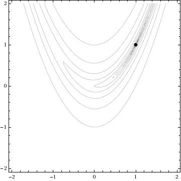
The global minimum of the Rosenbrock function lies at the point x=1, y=1 and is shown in the above diagram by a black spot. Note that the contours are not evenly spaced in this diagram – they are logarithmically spaced instead so the solution lies inside a very deep, narrow, banana shaped valley. The distinctive shape of this function’s contour lines is the reason for its alternative name – “Rosenbrock’s banana function”.

The valley causes a lot of problems for search algorithms such as the method of steepest descents which will quickly find the ‘entrance’ to the valley and then spend hundreds of iterations zigzagging from one side of it to the other – making very slow progress towards the minimum itself.

There is a Mathematica function called FindMinimum that can handle this kind of optimization problem and I wondered how its methods would handle the Rosenbrock function. In the back of my mind I thought that I might also be able to make a nice Wolfram Demonstration from the investigation. While looking at the documentation for FindMinimum I found an example that pretty much solved the problem for me.

pts = Reap[FindMinimum[(1 – x)^2 + 100 (-x^2 – y)^2, {{x, -1.2}, {y, 1}}, StepMonitor :> Sow[{x, y}]]][[2, 1]];
pts = Join[{{-1.2, 1}}, pts];

This finds the minimum point from a starting point of x=-1.2, y=1 and also stores all of the intermediate steps so you can see the path that Mathematica takes in looking for the solution. The only other piece of information needed was to find out how to specify the solution method. It turns out that this is obvious – just use the option

Method->”MethodNameHere”

replacing MethodNameHere with whatever method you want Mathematica to use. You can choose from ConjugateGradient, LevenbergMarquardt, Newton, QuasiNewton, PrincipalAxis and InteriorPoint.

All that remained was to wrap this up in a Manipulate statement, make it look pretty, add some controls and submit it to the demonstrations project. The result can be found here.

One of the things I like about the process of submitting demonstrations to the project is that they are refereed. Someone will take the time to look at your code and make suggestions and small modifications before it gets published. This reduces the possibility of mistakes being made in the final version and really helps with the learning process. Almost every time I have submitted something, I have learned a little more about Mathematica – and that’s really the main reason for me doing it (well its also fun to have your name “up in lights” if I am being honest).

At this point I would like to thank the members of the Wolfram Demonstrations team who have dealt with my submissions so far – not only have they been a pleasure to work with and extremely patient but they have also spared my blushes by pointing out some very stupid mistakes in my code. Of course any that remain are my fault and not theirs.

In a recent post I asked if anyone had any requests for any Wolfram Demonstrations that they would like to see made. Maria Andersen of the Teaching College Math Technology Blog requested a demonstration that would produce music from the decimal expansion of rational numbers in the same way that this one does for irrational numbers. Well, I always aim to please so here it is:

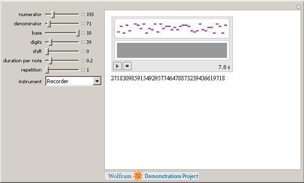
Just set the numerator and denominator with the sliders, choose the base of the result, the number of digits etc, along with what instrument you want and then click play. Remember, if you don’t have Mathematica then you can always use their free MathPlayer to run this demonstration. I hope this is what you were looking for Maria but if it isn’t then let me know what you would like changed and I will see what I can do.

If anyone else has any Wolfram Demonstration requests then leave a comment and I might just code it up for you (unless someone beats me to it of course).

Next Friday will be March 14th which is celebrated by some as Pi Day since the date is 3/14 in American date format and the first three digits of Pi are 3.14 (as if I have to tell you!). One or two people have been looking for inspiration as to what to do for Pi Day in schools and I thought that it would be fun to write a Wolfram Demonstration especially for Pi Day, after all, my Valentine’s day demonstrations turned out to be quite popular.

So the question that remained to be answered was “what demonstration should I write?”

I have already written a post about making music out of the digits of Pi and discovered that a great demonstration had been written by Hector Zenil so there was no point in thinking about that.

How about Buffon’s needle? That’s a fun problem that leads to an approximation of Pi. Unfortunately for me – this is a demonstration that has already been written.

Perhaps I could do something that looked at the randomness in the digits of Pi? After all – this blog IS called walking randomly and I haven’t looked at randomness very much yet. Unfortunately I have been beaten to this one too (By Stephen Wolfram himself no less).

My next thought was to consider some series that would sum up to approximations of Pi. Again – it’s been done.

In addition to these three there are many others such as

• Consecutive Digits in the Expansion of Pi
• Pi Digits Bar Chart
• Pi Digits Pie
• Wallis’ Sieve Pi Approximation
• Graphs Of Successive Digits Of Pi, E and Phi
• Wallis Formula

That’s a lot of Pi and I have only just gotten started. All in all I am stumped – I have no idea of a demonstration I might write for Pi Day but if you can think of something then let me know and I will see what I can do :) (Oh and I will make sure that you get credit for your idea when I submit it to the project)