Walking Randomly

Some time ago now, Sam Shah of Continuous Everywhere but Differentiable Nowhere fame discussed the standard method of obtaining the square root of the imaginary unit, i, and in the ensuing discussion thread someone asked the question “What is i^i – that is what is i to the power i?”

Sam immediately came back with the answer e^(-pi/2) = 0.207879…. which is one of the answers but as pointed out by one of his readers, Adam Glesser, this is just one of the infinite number of potential answers that all have the form e^{-(2k+1) pi/2} where k is an integer. Sam’s answer is the principle value of i^i (incidentally this is the value returned by google calculator if you google i^i – It is also the value returned by Mathematica and MATLAB). Life gets a lot more complicated when you move to the complex plane but it also gets a lot more interesting too.

While on the train into work one morning I was thinking about Sam’s blog post and wondered what the principal value of i^i^i (i to the power i to the power i) was equal to. Mathematica quickly provided the answer:

N[I^I^I]
0.947159+0.320764 I

So i is imaginary, i^i is real and i^i^i is imaginary again. Would i^i^i^i be real I wondered – would be fun if it was. Let’s see:

N[I^I^I^I]
0.0500922+0.602117 I

gah – a conjecture bites the dust – although if I am being honest it wasn’t a very good one.  Still, since I have started making ‘power towers’ I may as well continue and see what I can see. Why am I calling them power towers? Well, the calculation above could be written as follows:

As I add more and more powers, the left hand side of the equation will tower up the page….Power Towers.  We now have a sequence of the first four power towers of i:

i = i
i^i = 0.207879
i^i^i = 0.947159 + 0.32076 I
i^i^i^i = 0.0500922+0.602117 I

Sequences of power towers

“Will this sequence converge or diverge?”, I wondered.  I wasn’t in the mood to think about a rigorous mathematical proof, I just wanted to play so I turned back to Mathematica.  First things first, I needed to come up with a way of making an arbitrarily large power tower without having to do a lot of typing.  Mathematica’s Nest function came to the rescue and the following function allows you to create a power tower of any size for any number, not just i.

tower[base_, size_] := Nest[N[(base^#)] &, base, size]

Now I can find the first term of my series by doing

In[1]:= tower[I, 0]

Out[1]= I

Or the 5th term by doing

In[2]:= tower[I, 4] 

Out[2]= 0.387166 + 0.0305271 I

To investigate convergence I needed to create a table of these. Maybe the first 100 towers would do:

ColumnForm[
 Table[tower[I, n], {n, 1, 100}]
 ]

The last few values given by the command above are

0.438272+ 0.360595 I
0.438287+ 0.360583 I
0.438287+ 0.3606 I
0.438275+ 0.360591 I
0.438289+ 0.360588 I

Now this is interesting – As I increased the size of the power tower, the result seemed to be converging to around 0.438 + 0.361 i. Further investigation confirms that the sequence of power towers of i converges to 0.438283+ 0.360592 i.  If you were to ask me to guess what I thought would happen with large power towers like this then I would expect them to do one of three things – diverge to infinity, stay at 1 forever or quickly converge to 0 so this is unexpected behaviour (unexpected to me at least).

They converge, but how?

My next thought was ‘How does it converge to this value?  In other words, ‘What path through the complex plane does this sequence of power towers take?”  Time for a graph:

tower[base_, size_] := Nest[N[(base^#)] &, base, size];
complexSplit[x_] := {Re[x], Im[x]};
ListPlot[Map[complexSplit, Table[tower[I, n], {n, 0, 49, 1}]],
 PlotRange -> All]

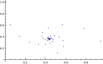
Who would have thought you could get a spiral from power towers? Very nice! So the next question is ‘What would happen if I took a different complex number as my starting point?’ For example – would power towers of (0.5 + i) converge?’

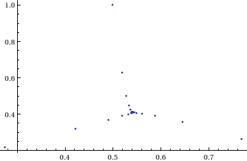
The answer turns out to be yes – power towers of (0.5 + I) converge to 0.541199+ 0.40681 I but the resulting spiral looks rather different from the one above.

tower[base_, size_] := Nest[N[(base^#)] &, base, size];
complexSplit[x_] := {Re[x], Im[x]};
ListPlot[Map[complexSplit, Table[tower[0.5 + I, n], {n, 0, 49, 1}]],
 PlotRange -> All]

The zoo of power tower spirals

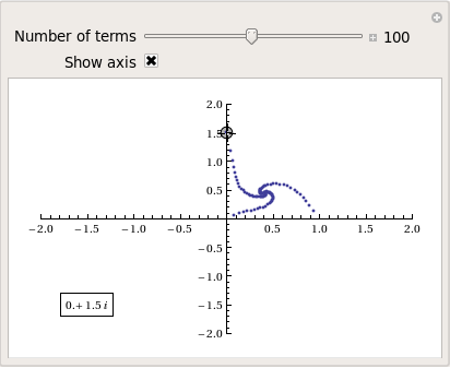
So, taking power towers of two different complex numbers results in two qualitatively different ‘convergence spirals’. I wondered how many different spiral types I might find if I consider the entire complex plane?  I already have all of the machinery I need to perform such an investigation but investigation is much more fun if it is interactive.  Time for a Manipulate

complexSplit[x_] := {Re[x], Im[x]};

tower[base_, size_] := Nest[N[(base^#)] &, base, size];

generatePowerSpiral[p_, nmax_] :=
  Map[complexSplit, Table[tower[p, n], {n, 0, nmax-1, 1}]];

Manipulate[const = p[[1]] + p[[2]] I;
 ListPlot[generatePowerSpiral[const, n],
 PlotRange -> {{-2, 2}, {-2, 2}}, Axes -> ax,
 Epilog -> Inset[Framed[const], {-1.5, -1.5}]], {{n, 100,
 "Number of terms"}, 1, 200, 1,
 Appearance -> "Labeled"}, {{ax, True, "Show axis"}, {True,
 False}}, {{p, {0, 1.5}}, Locator}]

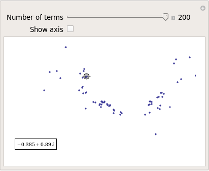
After playing around with this Manipulate for a few seconds it became clear to me that there is quite a rich diversity of these convergence spirals. Here are a couple more

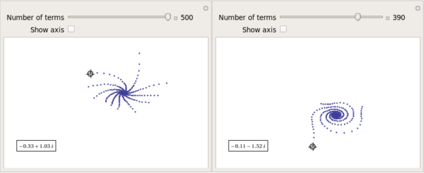
Some of them take a lot longer to converge than others and then there are those that don’t converge at all:

Optimising the code a little

Before I could investigate convergence any further, I had a problem to solve: Sometimes the Manipulate would completely freeze and a message eventually popped up saying “One or more dynamic objects are taking excessively long to finish evaluating……”  What was causing this I wondered?

Well, some values give overflow errors:

In[12]:= generatePowerSpiral[-1 + -0.5 I, 200]

General::ovfl: Overflow occurred in computation. >>
General::ovfl: Overflow occurred in computation. >>
General::ovfl: Overflow occurred in computation. >>
General::stop: Further output of General::ovfl will be suppressed during this calculation. >>

Could errors such as this be making my Manipulate unstable?  Let’s see how long it takes Mathematica to deal with the example above

AbsoluteTiming[ListPlot[generatePowerSpiral[-1  -0.5 I, 200]]]

On my machine, the above command typically takes around 0.08 seconds to complete compared to 0.04 seconds for a tower that converges nicely; it’s slower but not so slow that it should break Manipulate.  Still, let’s fix it anyway.

Look at the sequence of values that make up this problematic power tower

generatePowerSpiral[-0.8 + 0.1 I, 10]

{{-0.8, 0.1}, {-0.668442, -0.570216}, {-2.0495, -6.11826},
{2.47539*10^7,1.59867*10^8}, {2.068155430437682*10^-211800874,
-9.83350984373519*10^-211800875}, {Overflow[], 0}, {Indeterminate,
  Indeterminate}, {Indeterminate, Indeterminate}, {Indeterminate,
  Indeterminate}, {Indeterminate, Indeterminate}}

Everything is just fine until the term {Overflow[],0} is reached; after which we are just wasting time. Recall that the functions I am using to create these sequences are

complexSplit[x_] := {Re[x], Im[x]};
tower[base_, size_] := Nest[N[(base^#)] &, base, size];
generatePowerSpiral[p_, nmax_] :=
  Map[complexSplit, Table[tower[p, n], {n, 0, nmax-1, 1}]];

The first thing I need to do is break out of tower’s Nest function as soon as the result stops being a complex number and the NestWhile function allows me to do this.  So, I could redefine the tower function to be

tower[base_, size_] :=
 NestWhile[N[(base^#)] &, base, MatchQ[#, _Complex] &, 1, size]

However, I can do much better than that since my code so far is massively inefficient.  Say I already have the first n terms of a tower sequence; to get the (n+1)th term all I need to do is a single power operation but my code is starting from the beginning and doing n power operations instead.  So, to get the 5th term, for example, my code does this

I^I^I^I^I

instead of

(4th term)^I

The function I need to turn to is yet another variant of Nest – NestWhileList

fasttowerspiral[base_, size_] :=
 Quiet[Map[complexSplit,
 NestWhileList[N[(base^#)] &, base, MatchQ[#, _Complex] &, 1,
 size, -1]]];

The Quiet function is there to prevent Mathematica from warning me about the Overflow error.  I could probably do better than this and catch the Overflow error coming before it happens but since I’m only mucking around, I’ll leave that to an interested reader.  For now it’s enough for me to know that the code is much faster than before:

(*Original Function*)
AbsoluteTiming[generatePowerSpiral[I, 200];]

{0.036254, Null}

(*Improved Function*)
AbsoluteTiming[fasttowerspiral[I, 200];]

{0.001740, Null}

A factor of 20 will do nicely!

Making Mathematica faster by making it stupid

I’m still not done though. Even with these optimisations, it can take a massive amount of time to compute some of these power tower spirals. For example

spiral = fasttowerspiral[-0.77 - 0.11 I, 100];

takes 10 seconds on my machine which is thousands of times slower than most towers take to compute. What on earth is going on? Let’s look at the first few numbers to see if we can find any clues

In[34]:= spiral[[1 ;; 10]]

Out[34]= {{-0.77, -0.11}, {-0.605189, 0.62837}, {-0.66393,
  7.63862}, {1.05327*10^10,
  7.62636*10^8}, {1.716487392960862*10^-155829929,
  2.965988537183398*10^-155829929}, {1., \
-5.894184073663391*10^-155829929}, {-0.77, -0.11}, {-0.605189,
  0.62837}, {-0.66393, 7.63862}, {1.05327*10^10, 7.62636*10^8}}

The first pair that jumps out at me is {1.71648739296086210^-155829929, 2.96598853718339810^-155829929} which is so close to {0,0} that it’s not even funny! So close, in fact, that they are not even double precision numbers any more. Mathematica has realised that the calculation was going to underflow and so it caught it and returned the result in arbitrary precision.

Arbitrary precision calculations are MUCH slower than double precision ones and this is why this particular calculation takes so long. Mathematica is being very clever but its cleverness is costing me a great deal of time and not adding much to the calculation in this case. I reckon that I want Mathematica to be stupid this time and so I’ll turn off its underflow safety net.

SetSystemOptions["CatchMachineUnderflow" -> False]

Now our problematic calculation takes 0.000842 seconds rather than 10 seconds which is so much faster that it borders on the astonishing. The results seem just fine too!

When do the power towers converge?

We have seen that some towers converge while others do not. Let S be the set of complex numbers which lead to convergent power towers. What might S look like? To determine that I have to come up with a function that answers the question ‘For a given complex number z, does the infinite power tower converge?’ The following is a quick stab at such a function

convergeQ[base_, size_] :=
  If[Length[
     Quiet[NestWhileList[N[(base^#)] &, base, Abs[#1 - #2] > 0.01 &,
       2, size, -1]]] < size, 1, 0];

The tolerance I have chosen, 0.01, might be a little too large but these towers can take ages to converge and I’m more interested in speed than accuracy right now so 0.01 it is. convergeQ returns 1 when the tower seems to converge in at most size steps and 0 otherwise.:

In[3]:= convergeQ[I, 50]
Out[3]= 1

In[4]:= convergeQ[-1 + 2 I, 50]
Out[4]= 0

So, let’s apply this to a section of the complex plane.

towerFract[xmin_, xmax_, ymin_, ymax_, step_] :=
 ArrayPlot[
 Table[convergeQ[x + I y, 50], {y, ymin, ymax, step}, {x, xmin, xmax,step}]]
towerFract[-2, 2, -2, 2, 0.1]

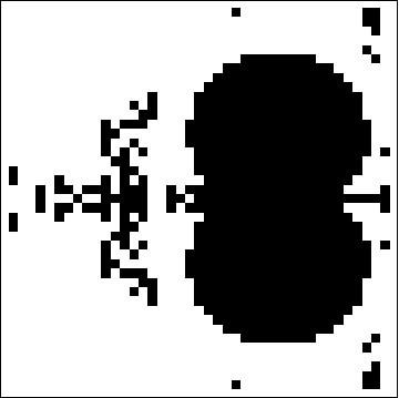
That looks like it might be interesting, possibly even fractal, behaviour but I need to increase the resolution and maybe widen the range to see what’s really going on. That’s going to take quite a bit of calculation time so I need to optimise some more.

Going Parallel

There is no point in having machines with two, four or more processor cores if you only ever use one and so it is time to see if we can get our other cores in on the act.

It turns out that this calculation is an example of a so-called embarrassingly parallel problem and so life is going to be particularly easy for us.  Basically, all we need to do is to give each core its own bit of the complex plane to work on, collect the results at the end and reap the increase in speed. Here’s the full parallel version of the power tower fractal code

(*Complete Parallel version of the power tower fractal code*)

convergeQ[base_, size_] :=
 If[Length[
 Quiet[NestWhileList[N[(base^#)] &, base, Abs[#1 - #2] > 0.01 &,
 2, size, -1]]] < size, 1, 0];

LaunchKernels[];
DistributeDefinitions[convergeQ];
ParallelEvaluate[SetSystemOptions["CatchMachineUnderflow" -> False]];

towerFractParallel[xmin_, xmax_, ymin_, ymax_, step_] :=
 ArrayPlot[
 ParallelTable[
 convergeQ[x + I y, 50], {y, ymin, ymax, step}, {x, xmin, xmax, step}
, Method -> "CoarsestGrained"]]

This code is pretty similar to the single processor version so let’s focus on the parallel modifications.  My convergeQ function is no different to the serial version so nothing new to talk about there.  So, the first new code is

LaunchKernels[];

This launches a set of parallel Mathematica kernels. The amount that actually get launched depends on the number of cores on your machine.  So, on my dual core laptop I get 2 and on my quad core desktop I get 4.

DistributeDefinitions[convergeQ];

All of those parallel kernels are completely clean in that they don’t know about my user defined convergeQ function. This line sends the definition of convergeQ to all of the freshly launched parallel kernels.

ParallelEvaluate[SetSystemOptions["CatchMachineUnderflow" -> False]];

Here we turn off Mathematica’s machine underflow safety net on all of our parallel kernels using the ParallelEvaluate function.

That’s all that is necessary to set up the parallel environment.  All that remains is to change Map to ParallelMap and to add the argument Method -> “CoarsestGrained” which basically says to Mathematica ‘Each sub-calculation will take a tiny amount of time to perform so you may as well send each core lots to do at once’ (click here for a blog post of mine where this is discussed further).

That’s all it took to take this embarrassingly parallel problem from a serial calculation to a parallel one.  Let’s see if it worked.  The test machine for what follows contains a T5800 Intel Core 2 Duo CPU running at 2Ghz on Ubuntu (if you want to repeat these timings then I suggest you read this blog post first or you may find the parallel version going slower than the serial one).  I’ve suppressed the output of the graphic since I only want to time calculation and not rendering time.

(*Serial version*)
In[3]= AbsoluteTiming[towerFract[-2, 2, -2, 2, 0.1];]
Out[3]= {0.672976, Null}

(*Parallel version*)
In[4]= AbsoluteTiming[towerFractParallel[-2, 2, -2, 2, 0.1];]
Out[4]= {0.532504, Null}

In[5]= speedup = 0.672976/0.532504
Out[5]= 1.2638

I was hoping for a bit more than a factor of 1.26 but that’s the way it goes with parallel programming sometimes. The speedup factor gets a bit higher if you increase the size of the problem though. Let’s increase the problem size by a factor of 100.

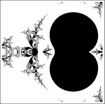
towerFractParallel[-2, 2, -2, 2, 0.01]

The above calculation took 41.99 seconds compared to 63.58 seconds for the serial version resulting in a speedup factor of around 1.5 (or about 34% depending on how you want to look at it).

Other optimisations

I guess if I were really serious about optimising this problem then I could take advantage of the symmetry along the x axis or maybe I could utilise the fact that if one point in a convergence spiral converges then it follows that they all do. Maybe there are more intelligent ways to test for convergence or maybe I’d get a big speed increase from programming in C or F#?  If anyone is interested in having a go at improving any of this and succeeds then let me know.

I’m not going to pursue any of these or any other optimisations, however, since the above exploration is what I achieved in a single train journey to work (The write-up took rather longer though). I didn’t know where I was going and I only worried about optimisation when I had to. At each step of the way the code was fast enough to ensure that I could interact with the problem at hand.

Being mostly ‘fast enough’ with minimal programming effort is one of the reasons I like playing with Mathematica when doing explorations such as this.

Treading where people have gone before

So, back to the power tower story. As I mentioned earlier, I did most of the above in a single train journey and I didn’t have access to the internet. I was quite excited that I had found a fractal from such a relatively simple system and very much felt like I had discovered something for myself. Would this lead to something that was publishable I wondered?

Sadly not!

It turns out that power towers have been thoroughly investigated and the act of forming a tower is called tetration. I learned that when a tower converges there is an analytical formula that gives what it will converge to:

Where W is the Lambert W function (click here for a cool poster for this function).  I discovered that other people had already made Wolfram Demonstrations for power towers too

• The Repeated Power function
• Convergence of a Hyperpower Sequence

There is even a website called tetration.org that shows ‘my’ fractal in glorious technicolor.  Nothing new under the sun eh?

Parting shots

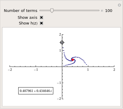
Well, I didn’t discover anything new but I had a bit of fun along the way. Here’s the final Manipulate I came up with

Manipulate[const = p[[1]] + p[[2]] I;
 If[hz,
  ListPlot[fasttowerspiral[const, n], PlotRange -> {{-2, 2}, {-2, 2}},
    Axes -> ax,
   Epilog -> {{PointSize[Large], Red,
      Point[complexSplit[N[h[const]]]]}, {Inset[
       Framed[N[h[const]]], {-1, -1.5}]}}]
  , ListPlot[fasttowerspiral[const, n],
   PlotRange -> {{-2, 2}, {-2, 2}}, Axes -> ax]
  ]
 , {{n, 100, "Number of terms"}, 1, 500, 1, Appearance -> "Labeled"}
 , {{ax, True, "Show axis"}, {True, False}}
 , {{hz, True, "Show h(z)"}, {True, False}}
 , {{p, {0, 1.5}}, Locator}
 , Initialization :> (
   SetSystemOptions["CatchMachineUnderflow" -> False];
   complexSplit[x_] := {Re[x], Im[x]};
   fasttowerspiral[base_, size_] :=
    Quiet[Map[complexSplit,
      NestWhileList[N[(base^#)] &, base, MatchQ[#, _Complex] &, 1,
       size, -1]]];
   h[z_] := -ProductLog[-Log[z]]/Log[z];
   )
 ]

and here’s a video of a zoom into the tetration fractal that I made using spare cycles on Manchester University’s condor pool.

If you liked this blog post then you may also enjoy:

• Simulating Harmonographs
• Polygonal numbers on quadratic number spirals
• The Unreasonable ineffectiveness of factoring
• Quadraflakes, Pentaflakes, Hexaflakes and more
• The equation that says Hi